MPI-AMRVAC 3.0: Updates to an open-source simulation framework
![aa45359-22-fig4[1]](https://www.tech-cc.eu/tcc/wp-content/uploads/2023/12/aa45359-22-fig41-678x381.jpg)
Received: 2 November 2022 Accepted: 12 March 2023
Abstract
Context. Computational astrophysics nowadays routinely combines grid-adaptive capabilities with modern shock-capturing, high resolution spatio-temporal integration schemes in challenging multidimensional hydrodynamic and magnetohydrodynamic (MHD) simulations. A large, and still growing, body of community software exists, and we provide an update on recent developments within the open-source MPI-AMRVAC code.
Aims. Complete with online documentation, the MPI-AMRVAC 3.0 release includes several recently added equation sets and offers many options to explore and quantify the influence of implementation details. While showcasing this flexibility on a variety of hydro-dynamic and MHD tests, we document new modules of direct interest for state-of-the-art solar applications.
Methods. Test cases address how higher-order reconstruction strategies impact long-term simulations of shear layers, with and without gas-dust coupling effects, how runaway radiative losses can transit to intricate multi-temperature, multiphase dynamics, and how different flavors of spatio-temporal schemes and/or magnetic monopole control produce overall consistent MHD results in combination with adaptive meshes. We demonstrate the use of super-time-stepping strategies for specific parabolic terms and give details on all the implemented implicit-explicit integrators. A new magneto-frictional module can be used to compute force-free magnetic field configurations or for data-driven time-dependent evolutions, while the regularized-Biot-Savart-law approach can insert flux ropes in 3D domains. Synthetic observations of 3D MHD simulations can now be rendered on the fly, or in post-processing, in many spectral wavebands.
Results. A particle module as well as a generic field line tracing module, fully compatible with the hierarchical meshes, can be used to do anything from sampling information at prescribed locations, to following the dynamics of charged particles and realizing fully two-way coupled simulations between MHD setups and field-aligned nonthermal processes. We provide reproducible, fully demonstrated tests of all code functionalities.
Conclusions. While highlighting the latest additions and various technical aspects (e.g., reading in datacubes for initial or boundary conditions), our open-source strategy welcomes any further code usage, contribution, or spin-off development.
Key words: hydrodynamics / magnetohydrodynamics (MHD) / methods: numerical / Sun: corona
Movies associated to Figs. 1, 3–5, 8, 9, 11, 19, 20 are available at https://www.aanda.org
© The Authors 2023
Open Access article, published by EDP Sciences, under the terms of the Creative Commons Attribution License (https://creativecommons.org/licenses/by/4.0), which permits unrestricted use, distribution, and reproduction in any medium, provided the original work is properly cited.
This article is published in open access under the Subscribe to Open model. Subscribe to A&A to support open access publication.
1 Introduction
Adaptive mesh refinement (AMR) is currently routinely available in many open-source, community-driven software efforts. The challenges associated with shock-dominated hydrodynamic (HD) simulations on hierarchically refined grids were already identified in the pioneering work by Berger & Colella (1989) and have since been carried over to generic frameworks targeting the handling of multiple systems of partial differential equations (PDEs). One such framework is the PARAMESH (MacNeice et al. 2000) package, which offers support for parallelized AMR on logically Cartesian meshes. Codes that inherited the PARAMESH AMR flexibility include the FLASH code, which started as pure hydro-AMR software for astrophysical applications (Fryxell et al. 2000). FLASH has since been used in countless studies, and a recent example includes its favorable comparison with an independent simulation study (Orban et al. 2022) that focused on modeling the challenging radiative-hydro behavior of a laboratory, laser-produced jet. PARAMESH has also been used in space-weather-related simulations in 3D ideal magnetohydrodynamics (MHD; Feng et al. 2012). For space weather applications, a similarly noteworthy forecasting framework employing AMR is discussed in Narechania et al. (2021), where Sun-to-Earth solar wind simulations in ideal MHD are validated. Another AMR package in active development is the CHOMBO library1, and this is how the PLUTO code (Mignone et al. 2012) inherits AMR functionality. Recent PLUTO additions showcase how dust particles can be handled using a hybrid particle-gas treatment (Mignone et al. 2019) and detail how novel nonlocal thermal equilibrium radiation hydro is performing (Colombo et al. 2019).
Various public-domain codes employ a native AMR implementation, such as the ENZO code (Bryan et al. 2014) or the RAMSES code, which started as an AMR-cosmological HD code (Teyssier 2002). In Astrobear (Cunningham et al. 2009), which is capable of using AMR on MHD simulations using constrained transport on the induction equation, the AMR functionality is known as the BEARCLAW package. Radiative MHD functionality for Astrobear, with a cooling function extending below 10000 K, was demonstrated in Hansen et al. (2018), who studied magnetized radiative shock waves. The AMR-MHD possibilities of NIRVANA have also been successfully increased (Ziegler 2005, 2008), and it has more recently added a chemistry-cooling module, described in Ziegler (2018). Another AMR-MHD code that pioneered the field was introduced as the BATS-R-US code (Powell et al. 1999), which is currently the main solver engine used in the space weather modeling framework described in Tóth et al. (2012). Its AMR functionality has been implemented in the block-adaptive-tree library (BATL), a Fortran-AMR implementation. This library shares various algorithmic details with the AMR implementation in MPI-AMRVAC, described in Keppens et al. (2012), whose 3.0 update forms the topic of this paper.
Meanwhile, various coding efforts anticipate the challenges posed by modern exascale high performance computing systems, such as that realized by the task-based parallelism now available in the Athena++ (Stone et al. 2020) effort. This code is in active use and development, with, for example, a recently added gasdust module (Huang & Bai 2022) that is similar to the gas-dust functionality available for MPI-AMRVAC (Porth et al. 2014). This paper documents the code’s novel options for implicit-explicit (IMEX) handling of various PDE systems and demonstrates its use for gas-dust coupling. GAMER-2, as presented in Schive et al. (2018), is yet another community effort that offers AMR and many physics modules, where graphics processing unit (GPU) acceleration in addition to hybrid OpenMP/MPI allows effective resolutions on the order of 10 0003. Even more visionary efforts in terms of adaptive simulations, where multiple physics modules may also be run concurrently on adaptive grid hierarchies, include the DISPATCH (Nordlund et al. 2018) and PATCHWORK (Shiokawa et al. 2018) frameworks. This paper serves to provide an updated account of the MPI-AMRVAC functionality. Future directions and potential links to ongoing new developments are provided in our closing discussion.
2 Open-source strategy with MPI-AMRVAC
With MPI-AMRVAC, we provide an open-source framework written in Fortran where parallelization is achieved by a (possibly hybrid OpenMP-) MPI implementation, where the block adaptive refinement strategy has evolved to the standard block-based quadtree-octree (2D-3D) organization. While originally used to evaluate efficiency gains affordable through AMR for multidimensional HD and MHD (Keppens et al. 2003), later applications focused on special relativistic HD and MHD settings (van der Holst et al. 2008; Keppens et al. 2012). Currently, the GitHub source version2 is deliberately handling Newtonian dynamics throughout, and we refer to its MPI-AMRVAC 1.0 version as documented in Porth et al. (2014), while an update to MPI-AMRVAC 2.0 is provided in Xia et al. (2018). A more recent guideline on the code usability to solve generic PDE systems (including reaction-diffusion models) is found in Keppens et al. (2021). Since MPI-AMRVAC 2.0, we have a modern library organization (using the code for 1D, 2D or 3D applications), have a growing number of automated regression tests in place, and provide a large number of tests or actual applications from published work under, for example, the tests/hd subfolder for all simulations using the hydro module src/hd. This ensures full compliance with all modern requirements on data reproducibility and data sharing.
Our open-source strategy already led to various noteworthy off-spins, where, for example, the AMR framework and its overall code organization got inherited to create completely new functionality: the Black Hole Accretion Code (BHAC3)from Porth et al. (2017; and its extensions; see, e.g., Bacchini et al. 2019; Olivares et al. 2019; Weih et al. 2020) realizes a modern general-relativistic MHD (GR-MHD) code, which was used in the GR-MHD code comparison project from Porth et al. (2019). In Ripperda et al. (2019a) the GR-MHD code BHAC got extended to handle GR-resistive MHD (GR-RMHD) where IMEX strategies handled stiff resistive source terms. We here document how various IMEX strategies can be used in Newtonian settings for MPI-AMRVAC 3.0. The hybrid OpenMP-MPI parallelization strategy was optimized for BHAC in Cielo et al. (2022), and we inherited much of this functionality within MPI-AMRVAC 3.0. Other, completely independent GR-MHD software efforts that derived from earlier MPI-AMRVAC variants include GR-AMRVAC by Meliani et al. (2016), the Gmunu code introduced in Cheong et al. (2021, 2022), or the NOVAs effort presented in Varniere et al. (2022).
The code is also used in the most recent update to the space weather modeling effort EUHFORIA4, introduced in Pomoell & Poedts (2018). In the ICARUS5 variant presented by Verbeke et al. (2022), the most time-consuming aspect of the prediction pipeline is the 3D ideal MHD solver that uses extrapolated magnetogram data for solar coronal activity at 0.1 AU, to then advance the MHD equations till 2 AU, covering all 360° longitudes, within a ±60° latitude band. This represents a typical use-case of MPI-AMRVAC functionality, where the user can choose a preferred flux scheme, the limiters, the many ways to automatically (de)refine on weighted, user-chosen (derived) plasma quantities, while adopting the radial grid stretching introduced in Xia et al. (2018) in spherical coordinates. In what follows, we provide an overview of current MPI-AMRVAC 3.0 functionality that may be useful for future users, or for further spin-off developments.
3 Available PDE systems
The various PDE systems available in MPI-AMRVAC 3.0 are listed in Table 1. These cover a fair variety of PDE types (elliptic, parabolic, but with an emphasis toward hyperbolic PDEs), and it is noteworthy that almost all modules can be exploited in 1D to 3D setups. They are all fully compatible with AMR and can be combined with modules that can meaningfully be shared between the many PDE systems. Examples of such shared modules include
- the particle module in src/particle, which we briefly discuss in Sect. 7.1,
- the streamline and/or field line tracing module in src/modules/mod_trace_field.t as demonstrated in Sect. 7.2,
- additional physics in the form of source terms for the governing equations, such as src/physics/mod_radiative_cooling.t to handle optically thin radiative cooling effects (see also Sect. 4.1.3), or src/physics/mod_thermal_conduction.t for thermal conduction effects, src/physics/mod_viscosity.t for viscous problems.
Table 1 provides references related to module usage, while some general guidelines for adding new modules can be found in Keppens et al. (2021). These modules share the code-parallelism, the grid-adaptive capacities and the various time-stepping strategies, for example the IMEX schemes mentioned below in Sect. 5. In the next sections, we highlight novel additions to the framework, with an emphasis on multidimensional (M)HD settings. Adding a physics module to our open-source effort can follow the instructions in doc/addmodule.md and the info in doc/contributing.md to ensure that auto-testing is enforced. The code’s documentation has two components: (1) the markup documents collected in the doc folder, which appear as html files on the code website6; and (2) the inline source code documentation, which gets processed by Doxygen7 to deliver full dependency trees and documented online source code.
Table 1Equation sets available in MPI-AMRVAC 3.0.
4 Schemes and limiters for HD and MHD
Most MPI-AMRVAC applications employ a conservative finite volume type discretization, used in each sub-step of a multistage time-stepping scheme. This finite volume treatment, combined with suitable (e.g., doubly periodic or closed box) boundary conditions ensures conservation properties of mass, momentum and energy as demanded in pure HD or ideal MHD runs. Available explicit time-stepping schemes include (1) a one-step forward Euler, (2) two-step variants such as predictor-corrector (midpoint) and trapezoidal (Heun) schemes, and (3) higher-order, multistep schemes. Our default three-, four- and five-step time integration schemes fall into the strong stability preserving (SSP) Runge-Kutta schemes (Gottlieb 2005), indicated as SSPRK(s, p), which involve s stages while reaching temporal order p. In that sense, the two-step Heun variant is SSPRK(2,2). In Porth et al. (2014), we provided all details of the three-step SSPRK(3,3), four-step SSPRK(4,3) and the five-step SSPRK(5,4) schemes, ensuring third-, third-, and fourth-order temporal accuracy, respectively. Tables 2 and 3 provide an overview of the choices in time integrators as well as the available shock-capturing spatial discretization schemes for the HD and MHD systems. The IMEX schemes are further discussed in Sect. 5. We note that Porth et al. (2014) emphasized that, instead of the standard finite volume approach, MPI-AMRVAC also allows for high-order conservative finite difference strategies (in the mod_finite_difference.t module), but these will not be considered explicitly here. Having many choices for spatiotemporal discretization strategies allows one to select optimal combinations depending on available computation resources, or on robustness aspects when handling extreme differences in (magneto-)thermodynamical properties. The code allows a higher than second-order accuracy to be achieved on smooth problems. In Porth et al. (2014), where MPI-AMRVAC 1.0 was presented, we reported on setups that formally achieved up to fourth-order accuracy in space and time. Figure 7 in that paper quantifies this for a 3D circularly polarized Alfvén wave test, while in the present paper, Fig. 10 shows third-order accuracy on a 1.75D MHD problem involving ambipolar diffusion. The combined spatio-temporal order of accuracy reachable will very much depend on the problem at hand (discontinuity dominated or not), and on the chosen combination of flux schemes, reconstructions, and source term treatments.
The finite-volume spatial discretization approach in each sub-step computes fluxes at cell volume interfaces, updating conservative variables stored as cell-centered quantities representing volume averages; however, when using constrained transport for MHD, we also have cell-face magnetic field variables. We list in Table 3 the most common flux scheme choices for the HD and MHD systems. In the process where fluxes are evaluated at cell edges, a limited reconstruction strategy is used – usually on the primitive variables – where two sets of cell interface values are computed for each interface: one employing a reconstruction involving mostly left, and one involving mostly right cell neighbors. In what follows, we demonstrate some of the large variety of higher-order reconstruction strategies that have meanwhile been implemented in MPI-AMRVAC. For explicit time integration schemes applied to hyperbolic conservation laws, temporal and spatial steps are intricately linked by the Courant-Friedrichs-Lewy (CFL) stability constraint. Therefore, combining high-order time-stepping and higher-order spatial reconstructions is clearly of interest to resolve subtle details. Thereby, different flux scheme and reconstruction choices may be used on different AMR levels. We note that our AMR implementation is such that the maximum total number of cells that an AMR run can achieve is exactly equal to the maximum effective grid resolution, if the refinement criteria enforce the use of the finest level grid on the entire domain. Even when a transition to domain-filling turbulence occurs – where triggering finest level grids all over is likely to happen, a gain in using AMR versus a fixed resolution grid can be important, by cost-effectively computing a transient phase. In Keppens et al. (2003), we quantified these gains for typical HD and MHD problems, and reported on efficiency gains by factors of 5 to 20, with limited overhead by AMR. Timings related to AMR overhead, boundary conditions, I/O, and actual computing are reported by MPI-AMRVAC in the standard output channel. For the tests discussed below, this efficiency aspect can hence be verified by rerunning the demo setups provided.
Table 2Time integration methods in MPI-AMRVAC 3.0, as implemented in mod_advance.t.
Table 3Choices for the numerical flux functions in MPI-AMRVAC 3.0, as implemented in mod_finite_volume.t.
4.1 Hydrodynamic tests and applications
The three sections below contain a 1D Euler test case highlighting differences due to the employed reconstructions (Sect. 4.1.1), a 2D hydro test without and with gas-dust coupling (Sect. 4.1.2), and a 2D hydro test where optically thin radiative losses drive a runaway condensation and fragmentation (Sect. 4.1.3). We note that the hydrodynamic hd module of MPI-AMRVAC could also be used without solving explicitly for the total (i.e., internal plus kinetic) energy density evolution, in which case an isothermal or polytropic closure is assumed. Physical effects that can be activated easily include solving the equations in a rotating frame, adding viscosity, external gravity, thermal conduction and optically thin radiative losses.
4.1.1 TVD versus WENO reconstructions
Many of the implemented reconstruction and/or limiter choices in MPI-AMRVAC are briefly discussed in its online documentation8. These are used when doing reconstructions on (usually primitive) variables from cell center to cell edge values, where their reconstructed values quantify local fluxes (on both sides of the cell face). They mostly differ in whether or not they ensure (1) the total variation diminishing (TVD) property on scalar hyperbolic problems or rather build on the essentially non-oscillatory (ENO) paradigm, (2) encode symmetry preservation, and (3) achieve a certain theoretical order of accuracy (second-order or higher possibilities). Various reconstructions with limiters are designed purely for uniform grids, others are compatible with nonuniform grid stretching. In the mod_limiter.t module, one currently distinguishes many types as given in Table 4. The choice of limiter impacts the stencil of the method, and hence the number of ghost cells used for each grid block in the AMR structure, as listed in Table 4. In MPI-AMRVAC, the limiter (as well as the discretization scheme) can differ between AMR levels, where one may opt for a more diffusive (and usually more robust) variant at the highest AMR levels.
Notes. The formal order of accuracy (on smooth solutions), the needed number of ghost cells, and suitable references are indicated as well.
The option to use higher-order weighted ENO (WENO) reconstruction variants has been added recently, and here we show their higher-order advantage using the standard 1D HD test from Shu & Osher (1989). This was run on a 1D domain comprised between x = −4.5 and x = 4.5, and since it is 1D only, we compared uniform grid high resolution (25600 points) with low resolution (256 points) equivalents. This “low resolution” is inspired by actual full 3D setups, where it is typical to use several hundreds of grid cells per dimension. The initial condition in density, pressure and velocity is shown in Fig. 1, along with the final solution at t = 1.8. A shock initially situated at x = −4 impacts a sinusoidally varying density field with left and right states as in

We used a Harten, Lax and van Leer (HLL) solver (Harten et al. 1983) in a three-step time integration, had zero gradient boundary conditions, and set the adiabatic index to γ = 1.4. In Fig. 2 we zoom in on the compressed density variation that trails the right-ward moving shock, where the fifth-order “wenozp5” limiter from Acker et al. (2016) is exploited in both high and low resolution. For comparison, low resolution third-order “cada3” (Čiada & Torrilhon 2009), third-order “weno3,” and seventh-order “weno7” (Balsara & Shu 2000) results show the expected behavior where higher-order variants improve the numerical representation of the shock-compressed wave train9.
Table 4Reconstructions with limiter choices in MPI-AMRVAC 3.0, as typically used in the cell-center-to-cell-face reconstructions.
4.1.2 2D Kelvin-Helmholtz: Gas and gas-dust coupling
The Kelvin-Helmholtz (KH) instability is ubiquitous in fluids, gases, and plasmas, and can cause intricate mixing. We here adopt a setup10 used in a recent study of KH-associated ionneutral de-couplings by Hillier (2019), where a reference high resolution HD run was introduced as well. We emphasize the effects of limiters in multidimensional hydro studies, by running the same setup twice, switching only the limiter exploited. We also demonstrate that MPI-AMRVAC can equally study the same processes in gas-dust mixtures, which is relevant, for example, in protoplanetary disk contexts.
2D KH and limiters
The domain (x, y) ∈ [−1.5, 1.5] × [−0.75, 0.75] uses a base resolution of 128×64 with 6 levels of refinement, and hence we achieve 4096×2048 effective resolution. This should be compared to the uniform grids used in Hillier (2019), usually at 2048×1024, but with one extreme run at 16384×8192. Their Fig. 1 shows the density field at a very late time (t = 50) in the evolution where multiple mergers and coalescence events between adjacent vortices led to large-scale vortices of half the box width, accompanied by clearly turbulent smaller-scale structures. The setup uses a sharp interface at y = 0, with
where ΔV = 0.2, together with a uniform gas pressure p0 = 1/γ where γ = 5/3. The vertical velocity is seeded by white noise with amplitude 10−3. However, the two runs discussed here use the exact same initial condition: the t = 0 data are first generated using a noise realization and this is used for both simulations. This demonstrates at the same time the code flexibility to restart from previously generated data files, needed to, for example, resume a run from a chosen snapshot, which can even be done on a different platform, using a different compiler. We note that the setup here uses a discontinuous interface at t = 0, which is known to influence and preselect grid-scale fine-structure in the overall nonlinear simulations. Lecoanet et al. (2016) discussed how smooth initial variations can lead to reproducible KH behavior (including viscosity), allowing convergence aspects to be quantified. This is not possible with the current setup, but one can adjust this setup to the Lecoanet et al. (2016) configuration and activate viscosity source terms.
We use a three-step time integrator, with periodic sides and closed up/down boundaries (the latter ensured by (a)symmetry conditions). We use the HLLC scheme (see the review by Toro 2019), known to improve the baseline HLL scheme (Harten et al. 1983) in the numerical handling of density discontinuities. In Fig. 3, we contrast two runs at times t = 20, 40 that only differ in the limiter exploited, the left column again uses the wenozp5 limiter (Acker et al. 2016), while at right the Venkatakrishnan (Venkatakrishnan 1995) limiter is used, which is a popular limiter on unstructured meshes. While both runs start from the same t = 0 data, it is clear how the nonlinear processes at play in KH mixing ultimately lead to qualitatively similar, but quantitatively very different evolutions. The limiter is activated from the very beginning due to the sharp interface setup, and the simulation accumulates differences at each timestep. We note that the wenozp5 run (left panels) clearly shows much more pronounced finer-scale structure than the “venk” run (right panels). Since the setup is using a discontinuous initial condition, some of the fine-structure is not necessarily physical (Lecoanet et al. 2016). If statistical properties specific to the turbulent substructures are of interest, one should exploit the higher-order reconstructions, and perform multiple runs at varying effective resolution to fully appreciate physical versus numerical effects. We note that we did not (need to) include any hyper-diffusive terms or treatments here.
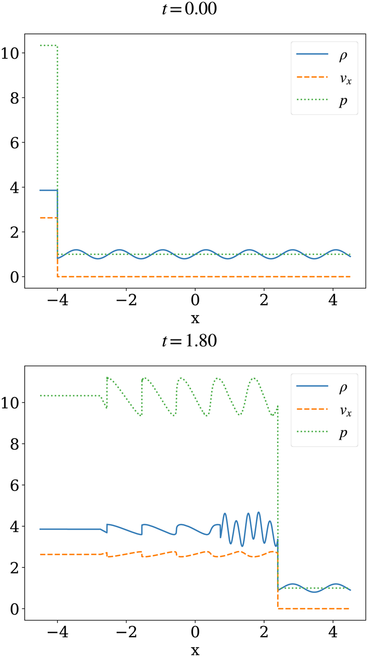 |
Fig. 1 ID Shu-Osher test. Shown are the density (solid blue line), velocity (dashed orange line), and pressure (dotted green line) for the initial time (top panel) and the final time (bottom panel). This high resolution numerical solution was obtained using the wenozp5 limiter. An animation is provided online. |
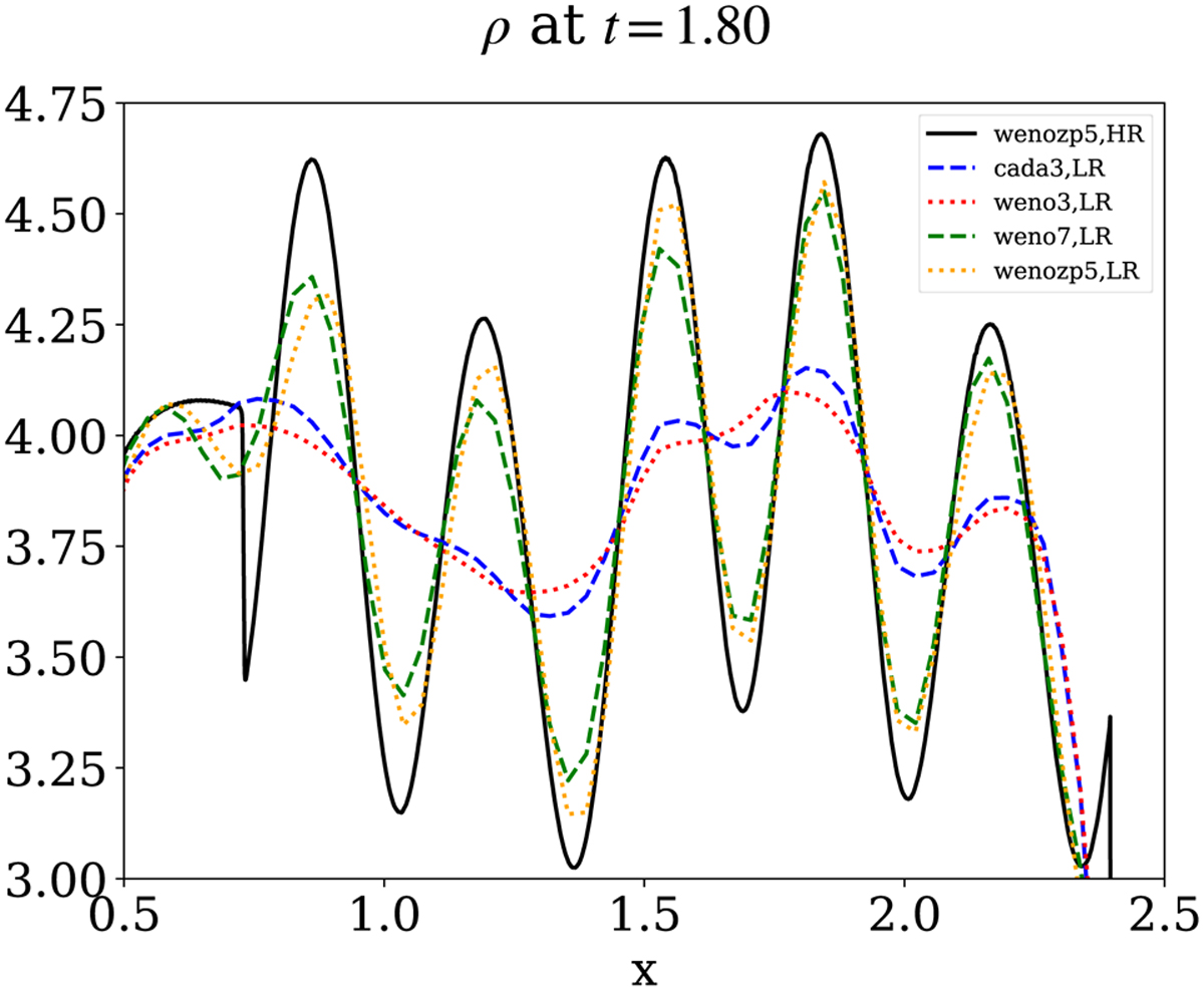 |
Fig. 2 ID Shu-Osher test. Comparison at final time t = 1.8 between different types of limiters at low resolution (LR) to the reference high resolution (HR) using the wenozp5 limiter (solid black) is shown. We zoom in on the density variation for x-axis values between 0.5 and 2.5 and ρ-values between 3 and 4.75. |
Gas-Dust KH evolutions
The HD module of MPI-AMRVAC provides the option to simulate drag-coupled gas-dust mixtures, introducing a user-chosen added number of dust species nd that differ in their “particle” size. In fact, every dust species is treated as a pressureless fluid, adding its own continuity and momentum equation for density ρdi and momentum ρdivdi, where interaction from dust species i ∈ 1… nd is typically proportionate to the velocity difference (v − vdi), writing ν for the gas velocity. This was demonstrated and used in various gas-dust applications (van Marle et al. 2011; Meheut et al. 2012; Hendrix & Keppens 2014; Porth et al. 2014; Hendrix et al. 2015, 2016). The governing equations as implemented are found in Porth et al. (2014), along with a suite of gas-dust test cases. We note that the dust species do not interact with each other, they only interact with the gas.
We here showcase a new algorithmic improvement specific to the gas-dust system: the possibility to handle the drag-collisional terms for the momentum equations through an implicit update. Thus far, all previous MPI-AMRVAC gas-dust simulations used an explicit treatment for the coupling, implying that the (sometimes very stringent and erratic) explicit stopping time criterion could slow down a gas-dust simulation dramatically. For Athena++, Huang & Bai (2022) recently demonstrated the advantage of implicit solution strategies allowing extremely short stopping time cases to be handled. In MPI-AMRVAC 3.0, we now provide an implicit update option for the collisional
terms in the momentum equations:
where we denote the end result of any previous (explicit) substage with T, Tdi. Noting that when the collisional terms are linear – that is, when we have the drag force fdi = αiρρdi (vdi − v) with a constant αi − an analytic implicit update can be calculated as follows:
 (4)
(4)
 (5)
(5)
Although the above is exact for any number of dust species nd when using proper expansions for dk, nk, and nik, in practice we implemented all terms up to the second order in Δt, implying that the expressions used are exact for up to two species (and approximate
for higher numbers), where we have
where ∀i = 1..nd we have
while
Equations (3) can be written in a compact form, where the already explicitly updated variables T enter the implicit stage:
 (9)
(9)
where
Following the point-implicit approach (see, e.g., Tóth et al. 2012), P(Un+1) is linearized in time after the explicit update,
 (11)
(11)
The elements of the Jacobian matrix ∂P/∂U contain in our case only elements of the form αiρdiρ. After the explicit update, the densities have already the final values at stage n + 1. Therefore, when αi is constant, the linearization is actually exact, but when αi also depends on the velocity, the implicit update might be less accurate.
The update of the gas energy density (being the sum of internal energy density eint and kinetic energy density) due to the collisions is done in a similar way and includes the frictional heating term,
This is different from the previous implementation, which only considered the work done by the momentum collisional terms (see Eq. (21) in Porth et al. 2014), but this added frictional heating term is generally needed for energy conservation (Braginskii 1965). The implicit update strategy can then be exploited in any multistage IMEX scheme.
As a demonstration of its use, we now repeat the KH run from above with one added dust species, where the dust fluid represents a binned dust particle size of [5 (b−1/2 − a−1/2) / (b−5/2 − a−5/2)]1/2 where a = 5 nm and b = 250 nm. We augment the initial condition for the gas with a dust velocity set identical to that of the gas by vx0d = vx0, but no velocity perturbation in the y-direction. The dust density is smaller than the gas density with a larger density contrast below and above the interface, setting ρ0d = Δρd for y > 0, ρ0d = 0.1 Δρd for y ≤ 0 where Δρd = 0.01. The time integrator used is a three-step ARS3 IMEX scheme, described in Sect. 5.
Results are shown in Fig. 4, for two different coupling regimes, which differ in the adopted constant coupling constant α, namely 100 and 1016. The associated explicit stopping time would scale with α−1, so larger α would imply very costly explicit in time simulations. Shown in Fig. 4 are the AMR grid structure in combination with the gas density variation at left (note that we here used different noise realizations at t = 0), as well as the single dust species density distribution at right, for t = 40. The density field for the dust shows similarly intricate fine-structure within the large-scale vortices that have evolved from multiple mergers. We used the same wenozp5 limiter as in the left panels of Fig. 3, and one may note how the gas dynamic vortex centers show clearly evacuated dust regions, consistent with the idealized KH gas-dust studies performed by Hendrix & Keppens (2014). The top versus bottom panels from Fig. 4 show that the AMR properly traces the regions of interest, the AMR criterion being based on density and temperature variables. The highly coupled case with α = 1016 can be argued to show more fine structure, as the collisions might have an effect similar to the diffusion for the scales smaller than the collisional mean free path (Popescu Braileanu et al. 2021). We note that Huang & Bai (2022) used corresponding α factors of 100 − 108 on their 2D KH test case, and did not investigate the very far nonlinear KH evolution we address here.
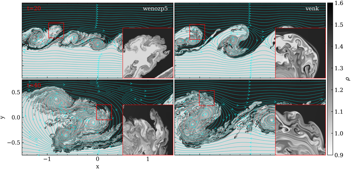 |
Fig. 3 Purely HD simulations of a 2D KH shear layer. The two runs start from the same initial condition and only deviate due to the use of two different limiters in the center-to-face reconstructions: wenozp5 (left column) and venk (right column). We show density views at times t = 20 (top row) and t= 40 (bottom row). The flow streamlines plotted here are computed by MPI-AMRVAC with its internal field line tracing functionality through the AMR hierarchy, as explained in Sect. 7.2. Insets show zoomed in views of the density variations in the red boxes, as indicated. An animation is provided online. |
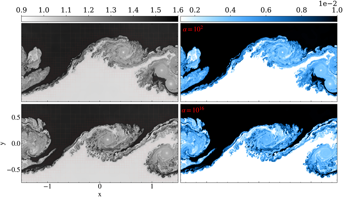 |
Fig. 4 As in Fig. 3, but this time in a coupled gas-dust evolution, at time t = 40, with one species of dust experiencing linear drag. In the top row, αdrag = 102, and the bottom row shows a much stronger drag coupling, αdrag = 1016. Left column: gas density. Right column: Dust density. The limiter used was wenozp5. An animation is provided online. |
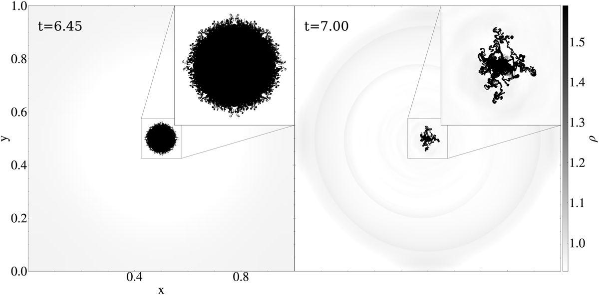 |
Fig. 52 D hydro runaway thermal condensation test. Density distributions are at times t = 6.45 (left) and t = 7 (right). The insets show zoomed-in views with more detail. An animation of this 2D hydro test is provided online. |
4.1.3 Thermally unstable evolutions
In many astrophysical contexts, one encounters complex multiphase physics, where cold and hot material coexist and interact. In solar physics, the million-degree hot corona is pervaded by cold (order 10000 K) condensations that appear as large-scale prominences or as more transient, smaller-scale coronal rain. Spontaneous in situ condensations can derive from optically thin radiative losses, and Hermans & Keppens (2021) investigated how the precise radiative loss prescription can influence the thermal instability process and its further nonlinear evolution in 2D magnetized settings. In practice, optically thin radiative losses can be handled by the addition of a localized energy sink term, depending on density and temperature, and MPI-AMRVAC provides a choice among 20 implemented cooling tables, as documented in the appendix of Hermans & Keppens (2021). The very same process of thermal instability, with its runaway condensation formation, is invoked for the so-called chaotic cold accretion (Gaspari et al. 2013) scenario onto black holes, or for the multiphase nature of winds and outflows in Active Galactic Nuclei (Waters et al. 2021), or for some of the fine-structure found in stellar wind-wind interaction zones (van Marle & Keppens 2012). Here, we introduce a new and reproducible test for handling thermal runaway in a 2D hydro setting. In van Marle & Keppens (2011), we inter-compared explicit to (semi)implicit ways for handling the localized source term, and confirmed the exact integration method of Townsend (2009) as a robust means to handle the extreme temperature-density variations that can be encountered. Using this method in combination with the SPEX_DM cooling curve Λ(T) (from Schure et al. 2009, combined with the low-temperature behavior as used by Dalgarno & McCray 1972), we set up a double-periodic unit square domain, resolved by a 64 × 64 base grid, and we allow for an additional 6 AMR levels. We use a five-step SSPRK(5,4) time integration, combined with the HLLC flux scheme, employing the wenozp5 limiter. We simulate until time t = 7, where the initial condition is a static (no flow) medium, of uniform pressure p = 1/γ throughout (with γ = 5/3). The density is initially ρ = 1.1 inside, and ρ = 1 outside of a circle of radius r = 0.15. To trigger this setup into a thermal runaway process, the energy equation not only has the optically thin ∝ ρ2Λ(T) sink term handled by the Townsend (2009) method, but also adds a special energy source term that balances exactly these radiative losses corresponding to the exterior ρ = 1 , p = 1 /γ settings. A proper implementation where ρ = 1 throughout would hence stay unaltered forever. Since the optically thin losses (and gains) require us to introduce dimensional factors (as Λ(T) requires the temperature T in Kelvin), we introduce units for length Lu = 109 cm, for temperature Tu = 106 K, and for number density nu = 109 cm−3. All other dimensional factors can be derived from these three.
As losses overwhelm the constant heating term within the circle r < 0.15, the setup naturally evolves to a largely spherically symmetric, constantly shrinking central density enhancement. This happens so rapidly that ultimately Rayleigh-Taylor-driven substructures form on the “imploding” density. Time t = 6.45 shown in Fig. 5 typifies this stage of the evolution, where one notices the centrally shrunk density enhancement, and fine structure along its entire edge. Up to this time, our implementation never encountered any faulty negative pressure, so no artificial bootstrapping (briefly discussed in Sect. 8.4) was in effect. However, to get beyond this stage, we did activate an averaging procedure on density-pressure when an isolated grid cell did result in unphysical pressure values below p < 10−14. Doing so, the simulation can be continued up to the stage where a more erratically behaving, highly dynamical and filamentary condensation forms, shown in the right panel of Fig. 5 at t = 7 (see also the accompanying movie). A similar HD transition – due to thermal instability and its radiative runaway – into a highly fragmented, rapidly evolving condensation is discussed in the appendix of Hermans & Keppens (2021), in that case as thermal runaway happens after interacting sound waves damp away due to radiative losses. An ongoing debate (e.g., McCourt et al. 2018; Gronke & Oh 2020) on whether this process is best described as “shattering” versus “splattering,” could perhaps benefit from this simple benchmark test11 to separate possible numerical from physical influences.
4.2 MHD tests and applications
The following three sections illustrate differences due to the choice of the MHD flux scheme (see Table 3) in a 2D ideal MHD shock-cloud setup (Sect. 4.2.1), differences due to varying the magnetic monopole control in a 2D resistive MHD evolution (Sect. 4.2.2), as well as a ID test showcasing ambipolar MHD effects on wave propagation through a stratified magnetized atmosphere (Sect. 4.2.3). We used this test to evaluate the behavior of the various super-time-stepping (STS) strategies available in MPI-AMRVAC for handling specific parabolic source additions. This test also employs the more generic splitting strategy usable in gravitationally stratified settings, also adopted recently in Yadav et al. (2022). We note that the mhd module offers many more possibilities than showcased here: we can, for example, drop the energy evolution equation in favor of an isothermal or polytropic closure, can ask to solve for internal energy density instead of the full (magnetic plus kinetic plus thermal) energy density, and have switches to activate anisotropic thermal conduction, optically thin radiative losses, viscosity, external gravity, as well as Hall and/or ambipolar effects.
4.2.1 Shock-cloud in MHD: Alfvén hits Alfvén
Shock-cloud interactions, where a shock front moves toward and interacts with a prescribed density variation, appear in many standard (M)HD code tests or in actual astrophysical applications. Here, we introduce an MHD shock-cloud interaction where an intermediate (also called Alfvén) shock impacts a cloud region that has a picture of Alfvén himself imprinted on it. This then simultaneously demonstrates how any multidimensional (2D or 3D) setup can initialize certain variables (in this case, the density at t = 0) in a user-selected area of the domain by reading in a separate, structured data set: in this case a vtk-file containing Alfvén’s image as a lookup table12 on a [0,1] × [0,1.5] rectangle. The 2D domain for the MHD setup takes (x, y) ∈ [−0.5,3] × [−1,2.5], and the pre-shock static medium is found where x > −0.3, setting ρ = 1 and p = 1/γ (γ = 5/3). The data read in from the image file are then used to change only the density in the subregion [0, 1] × [0, 1.5] to ρ = 1 + fsI(x, y) where a scale factor fs = 0.5 reduces the image I(x, y) range (containing values between 0 and 256, as usual for image data). We note that the regularly spaced input image values will be properly interpolated to the hierarchical AMR grid, and that this AMR hierarchy auto-adjusts to resolve the image at the highest grid level in use. The square domain is covered by a base grid of size 1282, but with a total of 6 grid levels, we achieve a finest grid cell of size 0.0008545 (to be compared to the 0.002 spacing of the original image).
To realize an Alfvén shock, a shock where the magnetic field lines flip over the shock normal (i.e., the By component changes sign across x = −0.3), we solved for the intermediate speed solution of the shock adiabatic, parametrized by three input values: (1) the compression ratio δ (here quantifying the post-shock density); (2) the plasma beta of the pre-shock region; and (3) the angle between the shock normal and the pre-shock magnetic field. Ideal MHD theory constrains δ ∈ [1, (γ + 1)/(γ − 1)], and these three parameters suffice to then compute the three admissible roots of the shock adiabatic that correspond to slow, intermediate and fast shocks (see, e.g., Gurnett & Bhattacharjee 2017). Selecting the intermediate root of the cubic equation then quantifies the upstream flow speed in the shock frame for a static intermediate shock. Shifting to the frame where the upstream medium is at rest then provides us with values for all post-shock quantities, fully consistent with the prevailing Rankine-Hugoniot conditions. In practice, we took δ = 2.5, an upstream plasma beta 2p/B2 = 0.1, and set the upstream magnetic field using a θ = 40° angle in the pre-shock region, with Bx = −B cos(θ) and By = Β sin(θ). This initial condition is illustrated in Fig. 6, showing the density as well as magnetic field lines. The shock-cloud impact is then simulated in ideal MHD till t = 1. Boundary conditions on all sides use continuous (zero gradient) extrapolation.
Since there is no actual (analytical) reference solution for this test, we ran a uniform grid case at 81922 resolution (i.e., above the effective 40962 achieved by the AMR settings). Figure 7 shows the density and the magnetic field structure at t = 1, where the HLLD scheme was combined with a constrained transport approach for handling magnetic monopole control. Our implementation of the HLLD solver follows Miyoshi & Kusano (2005) and Guo et al. (2016a), while divergence control strategies are discussed in the next section, Sect. 4.2.2. A noteworthy detail of the setup involves the corrugated appearance of a rightward-moving shock front that relates to a reflected shock front that forms at first impact. It connects to the original rightward moving shock in a triple point still seen for t = 1 at the top right (x, y) ≈ (2.6, 2.2). This density variation, shown also in a zoomed view in Fig. 7, results from a corrugation instability (that develops most notably beyond t = 0.7).
Figure 8 shows the final density distribution obtained with three different combinations of flux schemes, using AMR. We always employed a SSPRK(3,3) three-step explicit time marching with a “koren” limiter (Koren 1993), but varied the flux scheme from HLL, over HHLC, to HLLD. The HLL and HLLD variants used the hyperbolic generalized lagrange multiplier (or “glm”) idea from Dedner et al. (2002), while the HLLC run exploited the recently added multi-grid functionality for elliptic cleaning (see the next section and Teunissen & Keppens 2019). The density views shown in Fig. 8 are consistent with the reference result, and all combinations clearly demonstrate the corrugation of the reflected shock. We note that all the runs shown here did use a bootstrapping strategy (see Sect. 8.4) to recover automatically from local negative pressure occurrences (they occur far into the nonlinear evolution), where we used the averaging approach whenever one encounters a small pressure value below 10−7.
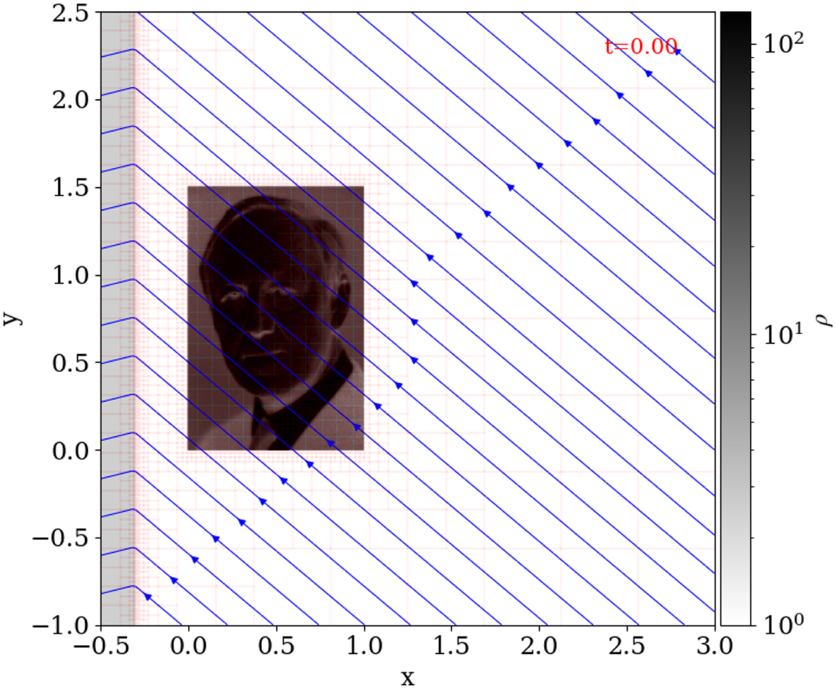 |
Fig. 6 Initial density variation for the 2D MHD Alfvén test: a planar Alfvén shock interacts with a density variation set from Alfvén’s image. The AMR block structure and magnetic field lines are overlaid in red and blue, respectively. |
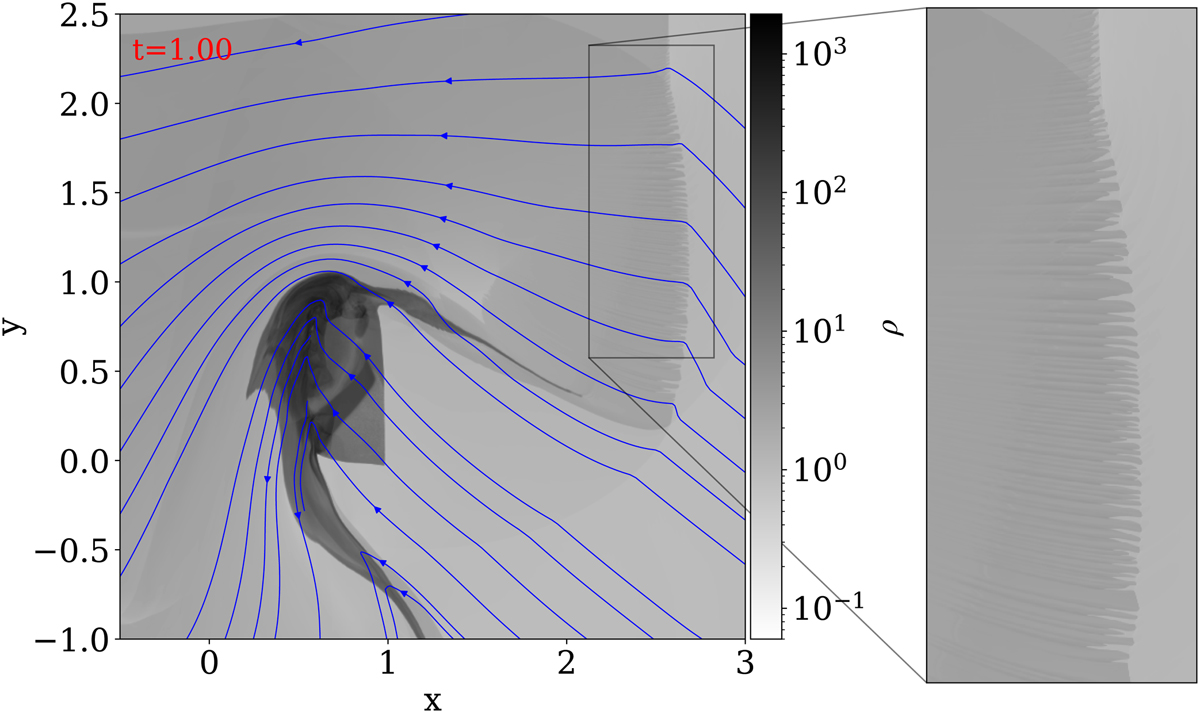 |
Fig. 7 Reference t = 1 uniform grid result for the Alfvén test using HLLD and constrained transport. The grid is uniform and 8192×8192. We show density and magnetic field lines, zooming in on the corrugated reflected shock at the right. |
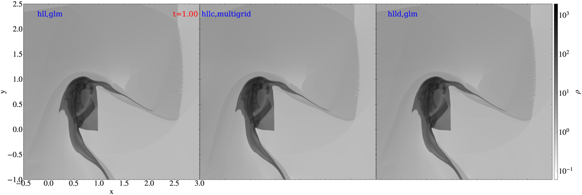 |
Fig. 8 Density view of the shock-cloud test, where an intermediate Alfvén shock impacts an “Alfvén” density field. Left: HLL and glm. Middle: HLLC and multigrid. Right: HLLD and glm. Compare this figure to the reference run from Fig. 7. An animation is provided online. |
4.2.2 Divergence control in MHD
Here, we simulate a 2D resistive MHD evolution that uses a uniform resistivity value η = 0.0001. The simulation exploits a (x, y) ∈ [−3, 3]2 domain, with base resolution 1282 but effective resolution 10242 (4 AMR levels). Always using a five-step SSPRK(5,4) time integration, the HLLC flux scheme, and an “mp5” limiter (Suresh & Huynh 1997), we simulate till t = 9 from an initial condition where an ideal MHD equilibrium is unstable to the ideal tilt instability. We use this test to show different strategies available for discrete magnetic monopole control, and how they lead to overall consistent results in a highly nonlinear, chaotic reconnection regime. This regime was used as a challenging test for different spatial discretizations (finite volume or finite differences) in Keppens et al. (2013), and shown to appear already at ten-fold higher η = 0.001 values.
The initial density is uniform ρ = 1 , while the pressure and magnetic field derive from a vector potential B = ∇ × A(r, θ)ez where (r, θ) denote local polar coordinates. In particular,
where r0 = 3.8317 denotes the first root of the Bessel function of the first kind, J1. This makes the magnetic field potential exterior to the unit circle, but non force-free within. An exact equilibrium where pressure gradient is balanced by Lorentz forces can then take the pressure as the constant value p0 = 1 /γ outside the unit circle, while choosing p = p0 + 0.5[r0A(r, θ)]2 within it. The constant was set to c = 2/(r0 J0(r0)). This setup produces two islands corresponding to antiparallel current systems perpendicular to the simulated plane, which repel. This induces a rotation and separation of the islands whenever a small perturbation is applied: this is due to the ideal tilt instability (also studied in Keppens et al. 2014). A t = 0 small perturbation is achieved by having an incompressible velocity field that follows v = ∇ × ϵ exp(−r2)ez with amplitude ϵ = 10−4.
This test case13 employs a special boundary treatment, where we extrapolate the primitive set of density, velocity components and pressure from the last interior grid cell, while both magnetic field components adopt a zero normal gradient extrapolation (i.e., a discrete formula yi = (−yi+2 + 4yi+1)/3 to fill ghost cells at a minimal edge, i.e., a left or bottom edge, and some analogous formula at maximal edges). This is done along all 4 domain edges (left, right, bottom, top). We note that ghost cells must ultimately contain correspondingly consistent conservative variables (density, momenta, total energy and magnetic field).
We use this test to highlight differences due to the magnetic monopole control strategy, for which MPI-AMRVAC 3.0 offers a choice between ten different options. These are listed in Table 5, along with relevant references. We note that we provide options to mix strategies (e.g., “lindeglm” both diffuses monopole errors in a parabolic fashion and uses an added hyperbolic variable to advect monopoles). There is a vast amount of literature related to handling monopole errors in combination with shock capturing schemes; for example, the seminal contribution by Tóth (2000) discusses this at length for a series of stringent ideal MHD problems. Here, we demonstrate the effect of three different treatments on a resistive MHD evolution where in the far nonlinear regime of the ideal tilt process, secondary tearing events can occur along the edges of the displaced magnetic islands. These edges correspond to extremely thin current concentrations, and the η = 0.0001 value ensures we can get chaotic island formation. We run the setup as explained above with three different strategies, namely “linde,” “multigrid,” and “ct.” The linde strategy was already compared on ideal MHD settings (a standard 2D MHD rotor and Orszag-Tang problem) in Keppens et al. (2003), while the constrained transport strategy is adopted in analogy to its implementation in the related GR-RMHD BHAC code (Olivares et al. 2019) with an additional option of using the contact-mode upwind constrained transport method by Gardiner & Stone (2005). We note that the use of ct requires us to handle the initial condition, as well as the treatment of the special boundary extrapolations, in a staggered-field tailored fashion, to ensure no discrete monopoles are present from initialization or boundary conditions. The multigrid method realizes the elliptic cleaning strategy as mentioned originally in Brackbill & Barnes (1980) on our hierarchical AMR grid. This uses a geometric multigrid solver to handle Poisson’s equation, ∇2ϕ = ∇ · Bbefore, followed by an update Bafter ← Bbefore − ∇ϕ, as described in Teunissen & Keppens (2019).
The evolution of the two spontaneously separating islands occurs identically for all three treatments, and it is noteworthy that all runs require no activation of a bootstrap strategy at all (i.e., they always produce positive pressure and density values). We carried out all three simulations up to t = 9, and our end time is shown in Fig. 9. The top panels show the density variations (the density was uniform initially), and one can see many shock fronts associated with the small-scale magnetic islands that appear. Differences between the three runs manifest themselves in where the first secondary islands appear, and how they evolve with time. This indicates how the 10242 effective resolution, combined with the SSPRK(5,4)-HLLD-mp5 strategy still is influenced by numerical discretization errors (numerical “resistivity”), although η = 0.0001. Relevant length scales of interest are the cross-sectional size of the plasmoids obtained, which should be resolved by at least several tens of grid cells. A related study of 2D merging flux tubes showing plasmoid formation (Ripperda et al. 2019b) in resistive, relativistic MHD setting, noted that effective resolutions beyond 80002 were needed to confidently obtain strict convergence at high Lundquist numbers.
We also plot the discrete divergence of the magnetic field in the bottom panels. Obviously, the rightmost ct variant realizes negligible (average absolute values at 10−12−10−11 throughout the entire evolution) divergence in its pre-chosen discrete monopole evaluation. Because of a slow accumulation of roundoff errors due to the divergence-preserving nature of the constrained transport method, this divergence can become larger than machine-precision zero, but remains very low. However, in any other discrete evaluation for the divergence, also the ct run displays monopole errors of similar magnitude and distribution as seen in both leftmost bottom panels of Fig. 9. Indeed, truncation-related monopole errors may approach unity in the thinning current sheets, at island edges, or at shock fronts. We note that the field lines as shown in the top panels have been computed by the code’s field-tracing module discussed in Sect. 7.2.
Table 5Options for ∇ · B control in MPI-AMRVAC 3.0.
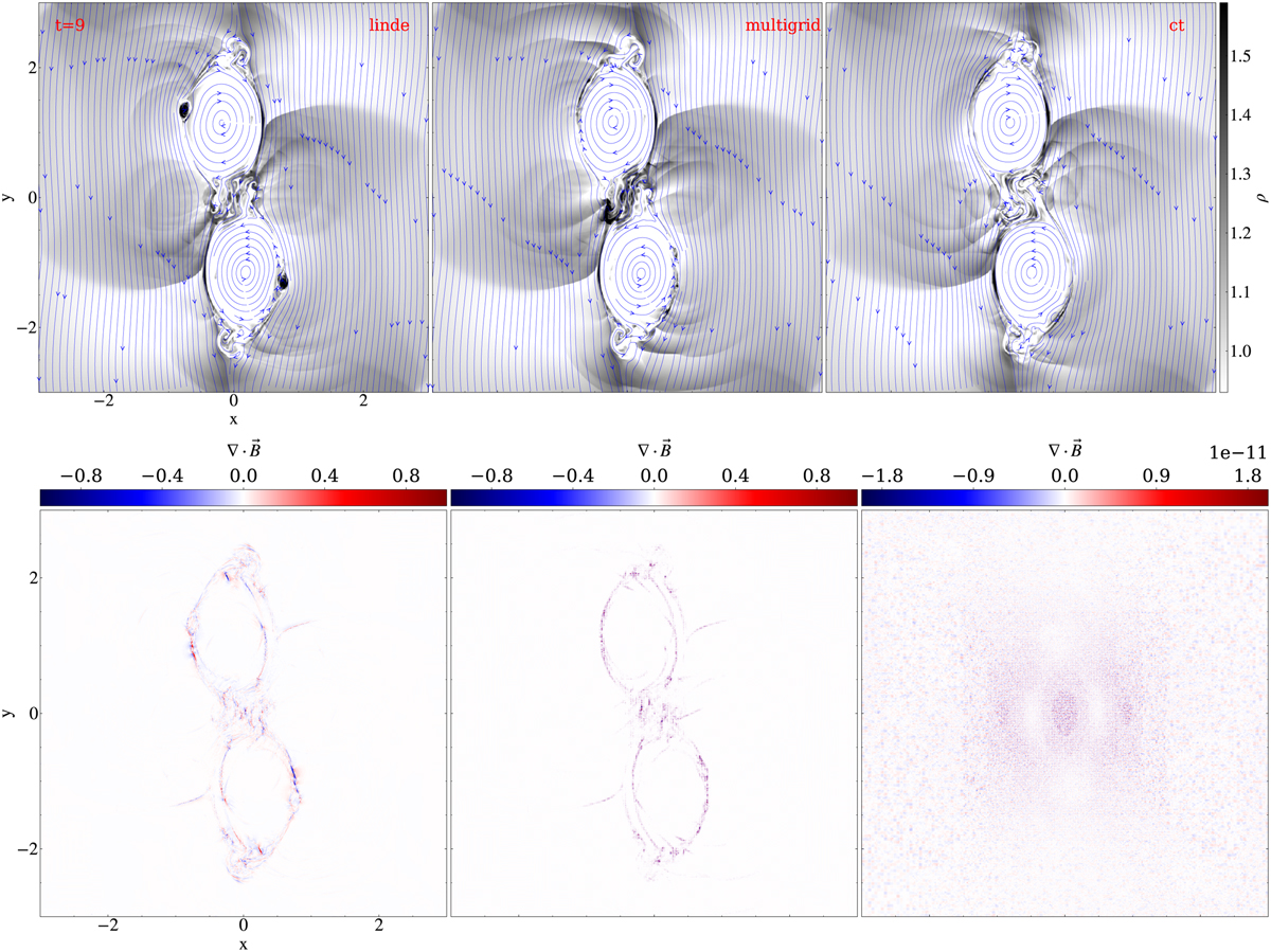 |
Fig. 9 Snapshots at time t = 9 for the 2D (resistive) MHD tilt evolution using, from left to right, different magnetic field divergence cleaning methods: linde, multigrid, and ct. First row: Density. The magnetic field lines are overplotted with blue lines, and, as in Fig. 3, they are computed by MPI-AMRVAC by field line tracing (see Sect. 7.2). Second row: Divergence of the magnetic field. An animation is provided online. |
4.2.3 Super-time-stepping and stratification splitting
In a system of PDEs, parabolic terms may impose a very small timestep for an explicit time advance strategy, as Δt ∝ Δx2, according to the CFL condition. In combination with AMR, this can easily become too restrictive. This issue can be overcome in practice by the STS technique, which allows the use of a relatively large (beyond the Δx2 restriction) explicit super-timestep Δts for the parabolic terms, by subdividing Δts into carefully chosen smaller sub-steps. This Δts can, for example, follow from the hyperbolic terms in the PDE alone, when parabolic and hyperbolic updates are handled in a split fashion. Super-time-stepping across Δts involves an s-stage Runge-Kutta scheme, and its number of stages s and the coefficients used in each stage get adjusted to ensure stability and accuracy. With the s-stage Runge-Kutta in a two-term recursive formulation, one can determine the sub-step length by writing the amplification factor for each sub-step as one involving an orthogonal family of polynomials that follow a similar two-term recursion. The free parameters involved can be fixed by matching the Taylor expansion of the solution to the desired accuracy. The use of either Chebyshev or Legendre polynomials gives rise to two STS techniques described in the literature: Runge-Kutta Chebyshev (RKC; Alexiades et al. 1996) and Runge-Kutta Legendre (RKL; Meyer et al. 2014). The second-order-accurate RKL2 variant was demonstrated on stringent anisotropic thermal conduction in multidimensional MHD settings by Meyer et al. (2014), and in MPI-AMRVAC, the same strategy was first used in a 3D prominence formation study (Xia & Keppens 2016) and a 3D coronal rain setup (Xia et al. 2017). We detailed in Xia et al. (2018) how the discretized parabolic term for anisotropic conduction best uses the slope-limited symmetric scheme introduced by Sharma & Hammett (2007), to preserve monotonicity. RKL1 and RKL2 variants are also implemented in Athena++ (Stone et al. 2020). RKC variants were demonstrated on Hall MHD and ambipolar effects by O’Sullivan & Downes (2006, 2007), and used for handling ambipolar diffusion in MHD settings in the codes MANCHA3D (González-Morales et al. 2018) and Bifrost (Nóbrega-Siverio et al. 2020).
The STS method eliminates the timestep restriction of explicit schemes and it is faster than standard sub-cycling. As pointed out in Meyer et al. (2014), compared to the RKC methods, the RKL variant ensures stability during every sub-step (instead of ensuring stability at the end of the super-time-step); have a larger stability region; do not require adjusting the final timestep (roundoff errors) and are more efficient (smaller number of sub-cycles). However, RKL methods require four times more storage compared to the RKC methods.
Meanwhile, both STS methods have been implemented in MPI-AMRVAC 3.0 and could be used for any parabolic source term. We specifically use STS for (anisotropic) thermal conductivity and ambipolar effects in MHD. The strategy can also be used for isotropic HD conduction or in the plasma component of a plasma-neutral setup. There are three splitting strategies to add the parabolic source term in MPI-AMRVAC: before the divergence of fluxes are added (referred to as “before”), after (“after”), or in a split (“split”) manner, meaning that the source is added for half a timestep before and half a timestep after the fluxes.
As a demonstration of the now available STS-usage for ambipolar effects, we perform a 1D MHD test of a fast wave traveling upward in a gravitationally stratified atmosphere where partial ionization effects are included through the ambipolar term. Due to this term, such a wave can get damped as it travels up. In the following, we tested both RKC and RKL methods combined with the three strategies before, after, and split for adding the source.
The setup is similar to that employed for a previous study of the ambipolar effect on MHD waves in a 2D setup in Popescu Braileanu & Keppens (2021). The MHD equations solved are for (up to nonlinear) perturbations only, where the variables distinguish between equilibrium (a hydrostatically stratified atmosphere with fixed pressure p0(z) and density ρ0(z)) and perturbed variables, as described in Yadav et al. (2022, see Eqs. (4)–(9)). The geometry adopted is 1.75 D (i.e., all three vector components are included, but only 1D z-variation is allowed). The background magnetic field is horizontal, with a small gradient in the magnetic pressure that balances the gravitational equilibrium. It is important to note that the ambipolar diffusion terms are essential in this test, in order to get wave damping, since a pure MHD variant would see the fast wave amplitude increase, in accord with the background stratification. Ambipolar damping gets more important at higher layers, as the adopted ambipolar diffusion coefficient varies inversely with density-squared. Popescu Braileanu & Keppens (2021) studied cases with varying magnetic field orientation, and made comparisons between simulated wave transformation behavior and approximate local dispersion relations. Here, we use a purely horizontal field and retrieve pure fast mode damping due to ambipolar diffusion.
We performed spatio-temporal convergence tests where we ran the simulation using an explicit implementation and 3200 grid points, having this as a reference solution. Left panel in Fig. 10 shows the reference numerical solution in its vertical velocity profile υz(z) at t = 0.7. This panel also over-plots the numerical solution for 3200 points for the six STS cases and we see how the seven solutions overlap. The right panel of Fig. 10 shows the normalized error,
as a function of the cell size Δz = {5 × 10⁻⁴, 2.5 × 10⁻⁴, 1.25 × 10⁻⁴, 6.25 × 10⁻⁵}, where u is the numerical solution obtained using STS and r is the reference numerical solution. Then we ran simulations using all six STS combinations using 3200, 1600, 800, and 400 points. We can observe that in all six cases the error curve is the same, and shows an order of convergence larger than 3. We used HLL flux scheme with a cada3 limiter (Čiada & Torrilhon 2009). The temporal scheme was a SSPRK(3,3) three-step explicit time.
Table 6 shows the computational cost of this simulation14, run with the same number of cores using an explicit implementation and the two variants of the STS technique. We can observe that when the STS technique is employed, the computational time drops by a factor of >10, being slightly smaller for RKC.
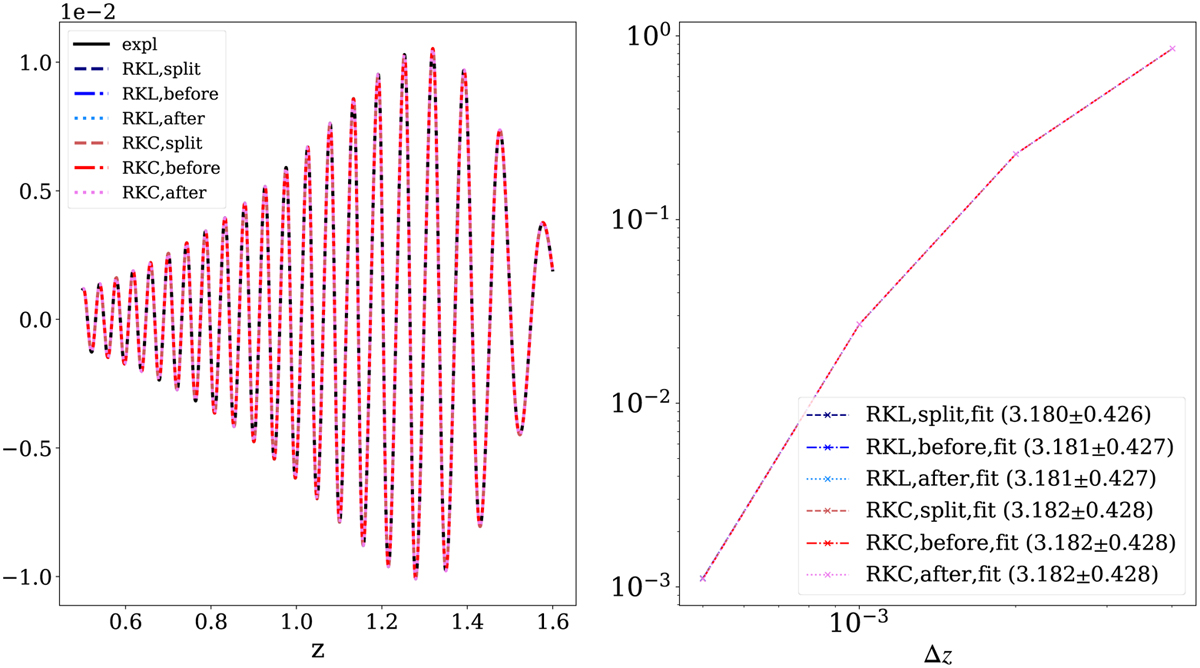 |
Fig. 10 1.75D ambipolar MHD wave test, where fast waves move upward against gravity. Left: vertical velocity profile for the two STS and three different splitting approaches and for an explicit reference run. Right: normalized error, 6, from Eq. (14) as a function of the cell size, comparing the numerical solution obtained using STS with a reference numerical solution obtained in an explicit implementation. All variants produce nearly identical results, such that all curves seem to be overlapping. |
Table 6Comparison of the computational times of explicit, RKL, and RKC methods (always exploiting eight cores).
5 IMEX variants
The generic idea of IMEX time integrators is to separate off all stiff parts for implicit evaluations, while handling all non-stiff parts using standard explicit time advancement. If we adopt the common (method-of-lines) approach where the spatial discretization is handled independently from the time dimension, we must time-advance equations of the form (15)
(15)
5.1 Multistep IMEX choices
One-step IMEX schemes
When we combine a first-order, single-step forward Euler (FE) scheme for the explicit part, with a first-order backward Euler (BE) scheme for the implicit part we arrive at an overall first-order accurate scheme, known as the IMEX Euler scheme. We can write the general strategy of this scheme as
and we can denote it by a combination of two Butcher tableaus, as follows:
Instead, the IMEX SP combination (with SP denoting a splitting approach), operates as follows: first do an implicit BE step, then perform an explicit FE step, as in
The above two schemes fall under the one-step strategy in MPI-AMRVAC, since only a single explicit advance is needed in each of them.
Two-step IMEX variants
A higher-order accurate IMEX scheme, given in Hundsdorfer & Verwer (2003, Eq. (4.12) of their chapter IV), is a combination of the implicit trapezoidal (or Crank-Nicholson) scheme and the explicit trapezoidal (or Heun) scheme, and writes as
This scheme is known as the IMEX trapezoidal scheme (sometimes denoted as IMEX CN, as it uses an implicit Crank-Nicholson step). Since it involves one implicit stage, and two explicit stages, while achieving second-order accuracy, the IMEX trapezoidal scheme is denoted as an IMEX(1,2,2) scheme. The IMEX Euler and IMEX SP are both IMEX (1,1,1).
The three IMEX(sim, sex, p) schemes given by Eqs. (16)–(18)–(20) differ in the number of stages used for the implicit (sim) versus explicit (sex) parts, and in the overall order of accuracy p. Both IMEX(1,1,1) first-order schemes from Eqs. (16)–(18) require one explicit stage, and one implicit one. The IMEX(1,2,2) trapezoidal scheme from Eq. (20) has one implicit stage, and two explicit ones. We can design another IMEX(1,2,2) scheme by combining the implicit midpoint scheme with a two-step explicit midpoint or Predictor-Corrector scheme. This yields the following double Butcher tableau,
and corresponds to the second-order IMEX midpoint scheme
Another variant of a two-step IMEX scheme available in MPI-AMRVAC is known as the IMEX222(λ) scheme from Pareschi & Russo (2005), where a λ parameter can be varied, but the default value  ensures that the scheme is SSP and L-stable (Izzo & Jackiewicz 2017). It has implicit evaluations at fractional steps λ and (1 − λ). Its double Butcher table reads
Three-step IMEX variants
Since we thus far almost exclusively handled Butcher tableaus with everywhere positive entries, we may prefer the IMEX-ARK(2,3,2) scheme (Giraldo et al. 2013), which also has two implicit stages, three explicit stages, at overall second order. It writes as
where we use the fixed values  while
while  .
.
Thus far, in terms of the double Butcher tableaus, we have mostly been combining schemes that have the same left column entries (i.e., sub-step time evaluations) for the implicit and the explicit stages. A possible exception was the FMEX222(λ) scheme. The implicit part was always in diagonally implicit Runge-Kutta type (or DIRK). Since one in practice implements the implicit stages separately from the explicit ones, one can relax the condition for implicit and explicit stages to be at the same time. In Rokhzadi et al. (2018) an IMEX-SSP(2,3,2) scheme with two implicit and three explicit stages was introduced, which indeed relaxes this; it is written as
If we allow for tableaus with also negative entries, we may even get third-order IMEX schemes, for example the ARS(2,3,3) scheme by Ascher et al. (1997; also denoted as IMEX-ARS3), where
which uses the fixed value  . This has the advantage of having only two implicit stages, which are usually more costly to compute than explicit stages. This ARS3 (Ascher et al. 1997) scheme has been shown to achieve better than second-order accuracy on some tests (Koto 2008), while needing three explicit and two implicit stages.
Finally, the IMEX-CB3a scheme, denoted as IMEXRKCB3a in Cavaglieri & Bewley (2015) uses three explicit steps, in combination with two implicit stages to arrive at overall third order, so it is an IMEX(2,3,3) variant:
The following relations fix all the values in its Butcher representation:
This scheme has the advantage that a low storage implementation (using 4 registers) is possible.
5.2 IMEX implementation and usage in MPI-AMRVAC
IMEX implementation
The various IMEX schemes are shared between all physics modules, and a generic implementation strategy uses the following pseudo-code ingredients for its efficient implementation. First, we introduced a subroutine,
which solves the (usually global) problem on the instantaneous AMR grid hierarchy given by (30)
(30)
This call leaves ub unchanged, and returns ua as the solution of this implicit problem. On entry, both states are available at time tn + βΔt. On exit, state ua is advanced by αΔt and has its boundary updated. Second,
just replaces the ua state with its evaluation (at time t) in the implicit part, that is, ua → Fim(t, ua). Finally, any explicit substep is handled by a subroutine,
which advances the ub state explicitly according to (31)
(31)
along with boundary conditions on ub(tb + αΔt).
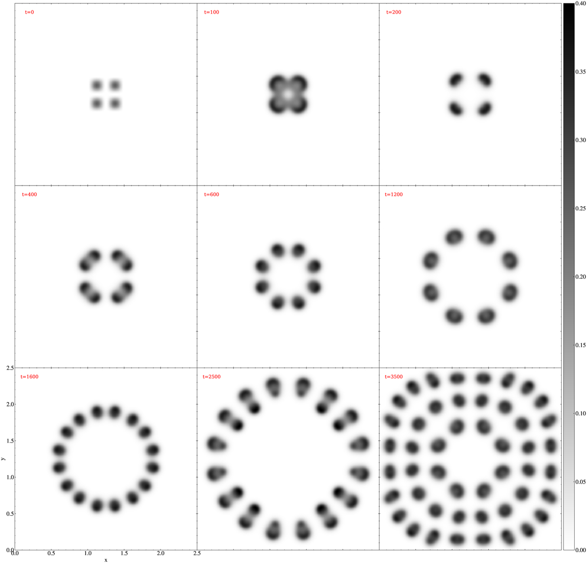 |
Fig. 11 Temporal evolution of υ(x, y, t) in a pure reaction-diffusion 2D Gray-Scott spot replication simulation. An animation is provided online. |
IMEX usage in MPI-AMRVAC
Currently, the IMEX schemes are used for handling (1) stiff diffusion terms, such as encountered in pure reaction-diffusion (or advection-reaction-diffusion) problems, or in the radiation-hydro module using flux-limited diffusion (FLD; Moens et al. 2022); (2) stiff coupling terms, such as in the gas-dust treatment as explained in Sect. 4.1.2, or in the ion-neutral couplings in the two-fluid module (Popescu Braileanu & Keppens 2022).
As an example of the first (handling stiff diffusion) IMEX use-case, we solve the pure reaction-diffusion 2D Gray-Scott spot replication simulation from Hundsdorfer & Verwer (2003; which also appears in Pearson 1993). The Gray-Scott two-component PDE system for u(x, t) = (u(x, t), υ(x, t)), has the following form: (32)
(32)
where F and k are positive constants; Du and Dυ are constant diffusion coefficients. We note that the feeding term F(1 − u) drives the concentration of u to one, whereas the term −(F + k)υ removes υ from the system. A wide range of patterns can be generated depending on the values of F and k (Pearson 1993), here we take F = 0.024 and k = 0.06. The diffusion coefficients have values D1 = 8 × 10⁻⁵ and D2 = 4 × 10⁻⁵. The initial conditions consist of a sinusoidal pattern in the center of the domain [0, 2.5]2:
Figure 11 shows the temporal evolution of υ(x, y, t) for a high resolution AMR simulation with a base resolution of 2562 cells. The five levels of refinement allow for a maximal effective resolution of 40962 cells. This long-term, high-resolution run then shows how the AMR quickly adjusts to the self-replicating, more volume-filling pattern that forms: while at t = 100 the coarsest grid occupies a large fraction of 0.859 of the total area, while the finest level covers only the central 0.066 area, this evolves to 0.031 (level 1) and 0.269 (level 5) at time t = 3500, the last time shown in Fig. 11. We note that on a modern 20-CPU desktop [using Intel Xeon Silver 4210 CPU at 2.20GHz], this entire run takes only 1053 s, of which less than 10 percent is spent on generating 36 complete file dumps in both the native .dat format, and the on-the-fly converted .vtu format (suitable for visualization packages such as ParaView or VisIt; see Sect. 8.5).
In order to perform a convergence study in time we take the same setup as Fig. 11, but for a uniform grid of 2562 cells (corresponding to a cell size of ≈0.012) and a final time tend = 100 (corresponding to the second panel of Fig. 11). We compare every simulation to a reference solution obtained with a classical fourth-order explicit Runge-Kutta scheme for Δt = 10−3. When explicitly solving the reaction-diffusion system corresponding to the initial conditions, the explicit timesteps are Δtd,expl = 0.149 and Δtr, expl = 5.803 associated with diffusion and the reaction terms, respectively. Hence, the use of the IMEX schemes reduces the computational cost by a factor of Δtr,expl /Δtd,expl ≈ 39 for this particular problem. For the convergence tests themselves the value of the largest timestep is fixed to unity, followed by four successive timesteps smaller by a factor of 2. The resulting convergence graph for Δt ∈ {0.0625, 0.125, 0.25, 0.5,1} is shown in Fig. 12, showing good correspondence between the theoretical and observed convergence rates.
We note that in this Gray-Scott problem15, the implicit update from Eq. (30) is actually a problem that can be recast to the following form:
and similarly for υ. For solving such generic elliptic problems on our AMR grid, we exploit the efficient algebraic multigrid solver as introduced in Teunissen & Keppens (2019).
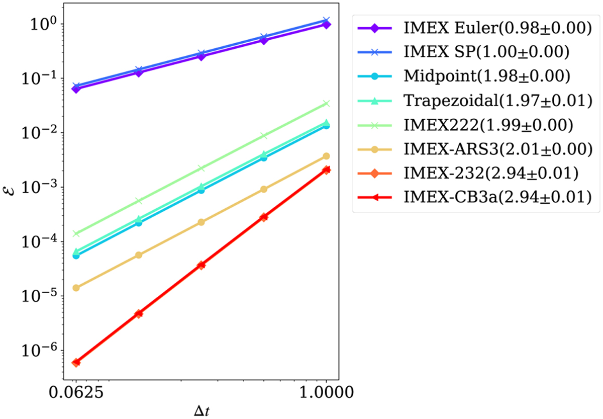 |
Fig. 12 Temporal convergence of the IMEX Runge-Kutta schemes in MPI-AMRVAC. The error computed as  , where N is the total number of grid points, is plotted as a function of the timestep used to obtain the numerical solutions u and υ using IMEX schemes. The uref and υref are the reference numerical solutions obtained using an explicit scheme with a much smaller timestep. , where N is the total number of grid points, is plotted as a function of the timestep used to obtain the numerical solutions u and υ using IMEX schemes. The uref and υref are the reference numerical solutions obtained using an explicit scheme with a much smaller timestep. |
6 Special (solar) physics modules
In recent years, MPI-AMRVAC has been actively applied to solar physics, where 3D MHD simulations are standard, although they may meet very particular challenges. Even when restricting attention to the solar atmosphere (photosphere to corona), handling the extreme variations in thermodynamic quantities (density, pressure and temperature) in combination with strong magnetic field concentrations, already implies large differences in plasma beta. Moreover, a proper handling of the chromo-spheric layers, along with the rapid temperature rise in a narrow transition region, really forces one to use advanced radiative-MHD treatments (accounting for frequency-dependent, nonlocal couplings between radiation and matter, true nonlocal-thermal-equilibrium physics affecting spectral line emission or absorption, etc.). Thus far, all these aspects are only handled approximately, with, for example, the recently added plasma-neutral src/twofl module (Popescu Braileanu & Keppens 2022) as an example where the intrinsically varying degree of ionization throughout the atmosphere can already be incorporated. To deal with large variations in plasma beta, we provided options to split off a time-independent (not necessarily potential) magnetic field B0 in up to resistive MHD settings (Xia et al. 2018), meanwhile generalized (Yadav et al. 2022) to split off entire 3D magneto-static force-balanced states −∇p0 + ρ0g + J0 × B0 = 0. For MHD and two-fluid modules, we add an option to solve internal energy equation instead of total energy equation to avoid negative pressure when plasma beta is extremely small.
A specific development relates to numerically handling energy and mass fluxes across the sharp transition region variation, which under typical solar conditions and traditional Spitzertype thermal conductivities can never be resolved accurately in multidimensional settings. Suitably modifying the thermal conduction and radiative loss prescriptions can preserve physically correct total radiative losses and heating aspects (Johnston et al. 2020). This led to the transition-region-adaptive-conduction (TRAC) approaches (Johnston et al. 2020, 2021; Iijima & Imada 2021; Zhou et al. 2021), with, for example, Zhou et al. (2021) introducing various flavors where the field line tracing functionality (from Sect. 7.2) was used to extend the originally 1D hydro incarnations to multidimensional MHD settings. Meanwhile, truly local variants (Iijima & Imada 2021; Johnston et al. 2021) emerged, and MPI-AMRVAC 3.0 provides multiple options16 collected in src/mhd/mod_trac.t. In practice, up to 7 variants of the TRAC method can be distinguished in higher dimensional (> 1D) setups, including the use of a globally fixed cut-off temperature, the (masked and unmasked) multidimensional TRACL and TRACB methods introduced in Zhou et al. (2021), or the local fix according to Iijima & Imada (2021).
Various modules are available that implement frequently recurring ingredients in solar applications. These are, for example: a potential-field-source-surface (PFSS) solution on a 3D spherical grid that extrapolates magnetic fields from a given bottom magnetogram (see src/physics/mod_pfss.t as evaluated in Porth et al. 2014), a method for extrapolating a magnetogram into a linear force-free field in a 3D Cartesian box (see src/physics/mod_lfff.t), or a modular implementation of the frequently employed 3D Titov-Démoulin (Titov & Démoulin 1999) analytic flux rope model (see src/physics/mod_tdfluxrope.t), or the functionality to perform nonlinear force-free field extrapolations from vector magnetograms (see src/physics/mod_magnetofriction.t as evaluated in Guo et al. 2016b,c).
In what follows, we demonstrate more recently added solarrelevant functionality, namely the addition of a time-dependent magneto-frictional (MF) module in Sect. 6.1, the possibility to insert flux ropes using the regularized Biot-Savart laws (RBSLs) from Titov et al. (2018) in Sect. 6.2, and the way to synthesize 3D MHD data to actual extreme ultraviolet (EUV) images in a simple on-the-fly fashion in Sect. 6.3.
6.1 Magneto-frictional module
The MF method is closely related to the MHD relaxation process (e.g., Chodura & Schlueter 1981). It is proposed by Yang et al. (1986) and considers both the momentum equation and the magnetic induction equation:
where ρ is the density, v the velocity, J = ∇ × B/μ0 the electric current density, B the magnetic field, p the pressure, g the gravitational field, ν the friction coefficient, and μ0 the vacuum permeability. To construct a steady-state force-free magnetic field configuration, the inertial, pressure-gradient, and gravitational forces are omitted in Eq. (35) and one only uses the simplified momentum equation to give the MF velocity:
Equations (36) and (37) are then combined together to relax an initially finite-force magnetic field to a force-free state where J × B = 0 with appropriate boundary conditions.
The MF method has been adopted to derive force-free magnetic fields in 3D domains (e.g., Roumeliotis 1996; Valori et al. 2005; Guo et al. 2016b,c). It is commonly regarded as an iteration process to relax an initial magnetic field that does not need to have an obvious physical meaning. For example, if the initial state is provided by an extrapolated potential field together with an observed vector magnetic field at the bottom boundary, the horizontal field components can jump discontinuously there initially, and locally are probably not in a divergence-free condition. The MF method can still relax this unphysical initial state to an almost force-free and divergence-free state (the degree of force-freeness and its solenoidal character can be quantified during the iterates and monitored). On the other hand, the MF method could also be used to actually mimic a time-dependent process (e.g., Yeates et al. 2008; Cheung & DeRosa 2012), although there are caveats about using the MF method in this way (Low 2013). The advantage of such a time-dependent MF method is that it consumes much less computational resources than a full MHD simulation to cover a long-term quasi-static evolution of nearly force-free magnetic fields. This allows us to simulate the global solar coronal magnetic field over a very long period, for instance, several months or even years.
We implemented a new MF module (src/mf), parallel to the existing physics modules like MHD, in MPI-AMRVAC. This module can be used in 2D and 3D, and in different geometries, fully compatible with (possibly stretched) block-AMR. We set the friction coefficient ν = ν0B2, where ν0 = 10−15 s cm−2 is the default value. The magnitude of the MF velocity is smoothly truncated to an upper limit υmax = 30 km s−1 by default to avoid extremely large numerical speed near magnetic null points (Pomoell et al. 2019). The ν0 and υmax are input parameters mf_nu and mf_vmax with dimensions. We allow a smooth decay of the MF velocity toward the physical boundaries to match line-tied quasi-static boundaries (Cheung & DeRosa 2012). In contrast to the previous MF module (still available as src/physics/mod_magnetofriction.t) used in Guo et al. (2016c), this new MF module in src/mf includes the time-dependent MF method and now fully utilizes the framework for data I/O with many more options of numerical schemes. Especially, the constrained transport scheme (Balsara & Spicer 1999), compatibly implemented with the staggered AMR mesh (Olivares et al. 2019), to solve the induction equation, Eq. (36), is recommended when using this new MF module. This then can enforce the divergence of magnetic field to near machine precision zero.
To validate the new MF module, we set up a test17, starting from a non-force-free bipolar twisted magnetic field (Mackay & van Ballegooijen 2001) to verify that the MF module can efficiently relax it to a force-free state. The magnetic field is given by
where B0 = 50 G is the peak flux density, β = 1 is a dimensionless parameter to control the twist of the magnetic field, and L0 = 10 Mm is the half distance between the peaks of two polarities on the z = 0 boundary. The test is performed in a 3D Cartesian box bounded by −40 ≤ x ≤ 40 Mm, −40 ≤ y ≤ 40 Mm, and 0 ≤ z ≤ 80 Mm with 4-level AMR grid of effective 256 × 256 × 256 resolution. The (MF) velocities in the ghost cells are set to zero. The induction equation is solved with a finite-volume scheme combining the HLL Riemann flux (Harten et al. 1983) with Čada’s third-order limiter (Čiada & Torrilhon 2009) for reconstruction and a three-step Runge-Kutta time integration. The magnetic field is extrapolated on the side and top boundaries assuming zero normal gradient. We compare two divergence control strategies, namely linde versus ct (from Table 5). In the run using linde, we use Courant number 0.3 for stability and a diffusive term in the induction equation diminishes the divergence of the magnetic field (Keppens et al. 2003). To keep the bottom magnetic flux distribution, the magnetic field vectors are fixed at the initial values in the first-layer (next to the physical domain) ghost cells of the bottom boundary and extrapolated to deeper layers of ghost cells with divergence-free condition. In the run ct, we use Courant number 0.8 and the constrained transport method with the initial face-centered magnetic field integrated from the edge-centered vector potential to start with zero numerical divergence of the magnetic field. The tangential electric field on the bottom surface is fixed to zero to preserve the magnetic flux distribution. Magnetic structures at the initial time 0 and the final time 900 are presented by magnetic field lines in Figs. 13a,b, respectively. The initial torus-like flux tube expands and relaxes to a twisted flux rope wrapped by sheared and potential arcades. In Figs. 13c,d, we present the force-free degree by the weighted average of the sine of the angle between the magnetic field and the current density as Eq. (13) of Guo et al. (2016c) and the divergence-free degree by the average dimensionless ∇ · B as the Eq. (11) of Guo et al. (2016c), respectively. In the ct run, the force-free degree rapidly decreases from 0.76 to lower than 0.1 within time 84, and converges to 0.0095. The divergence-free degree levels off to 1.5 × 10⁻¹⁴. In the run using linde, the force-free degree decreases similarly until 0.6 and slowly converges to a worse value of 0.16. The divergence-free degree quickly reaches a peak value of 0.098 and decreases to 1.5 × 10⁻⁴. Further investigation locates the large ∇ · B errors at the two main polarities in the first-layer cells above the bottom boundary in the linde run.
We also applied the new MF module to observations (provided in tests/mf/data_driven_tmf) for time-dependent evolution. Figure 14 shows an example of the application of the MF module in the solar active region 12673. We select the time range between 09:00 UT on 2017 September 3 and 15:00 UT on 2017 September 6 to do the simulation, which includes the buildup period for two X-class flares peaking at 09:10 UT (X2.2) and 12:02 UT (X9.3) on 2017 September 6, respectively. Solar Dynamics Observatory Helioseismic and Magnetic Imager (SDO/HMI) observes a temporal sequence of vector magnetic field on the photosphere. We use the SDO/HMI Active Region Patch (SHARP) data with a cadence of 12 min (Hoeksema et al. 2014). The series name of the data is “hmi.sharp_cea_720s.7115.” The vector velocity field is also derived by the inversion of the magnetic field using the differential affine velocity estimator for vector magnetograms (DAVE4VM; Schuck 2008). Then, both the temporal sequence of the vector magnetic field and the velocity field are used to fill the first-layer ghost cells at the bottom boundary to drive the evolution of the coronal magnetic field. The initial condition is a potential field at 09:00 UT on 2017 September 3 as shown in Fig. 14a. On a uniform (domain-decomposed) grid of 340 × 220 × 220 cells, the induction equation is solved with the same numerical schemes as in the linde run of the bipolar test. The magnetic field line evolution in Fig. 14 indicates that a twisted magnetic flux rope is formed along the polarity inversion line toward the explosion of the major flares. The resulting 3D magnetic field evolution can be compared to actual observations (in terms of their emission morphology), or can be used to start full 3D follow-up MHD simulations that incorporate actual plasma dynamics.
We note that we here did exploit linde divergence control, since the ct method requires a strict divergence-free boundary condition of magnetic field for numerical stability. For static cases (as in the much more idealized test from Fig. 13), this can be realized easily. However, for data-driven boundary conditions in which magnetic fields are directly given by actual observations, such strict divergence-free conditions cannot always be ensured. With the linde method, spurious divergence induced by a data-driven boundary can still be diffused and reduced, and the numerical scheme is stable even though locally the discrete divergence of magnetic field can be relatively large (as stated above for the test from Fig. 13, typically in the first grid cell layer). When we tried to apply the ct method to actual SDO data, code stability was compromised due to residual magnetic field divergence. Future work should focus on more robust, fully AMR-compatible means for performing data-driven runs using actual observational vector magnetic and flow data.
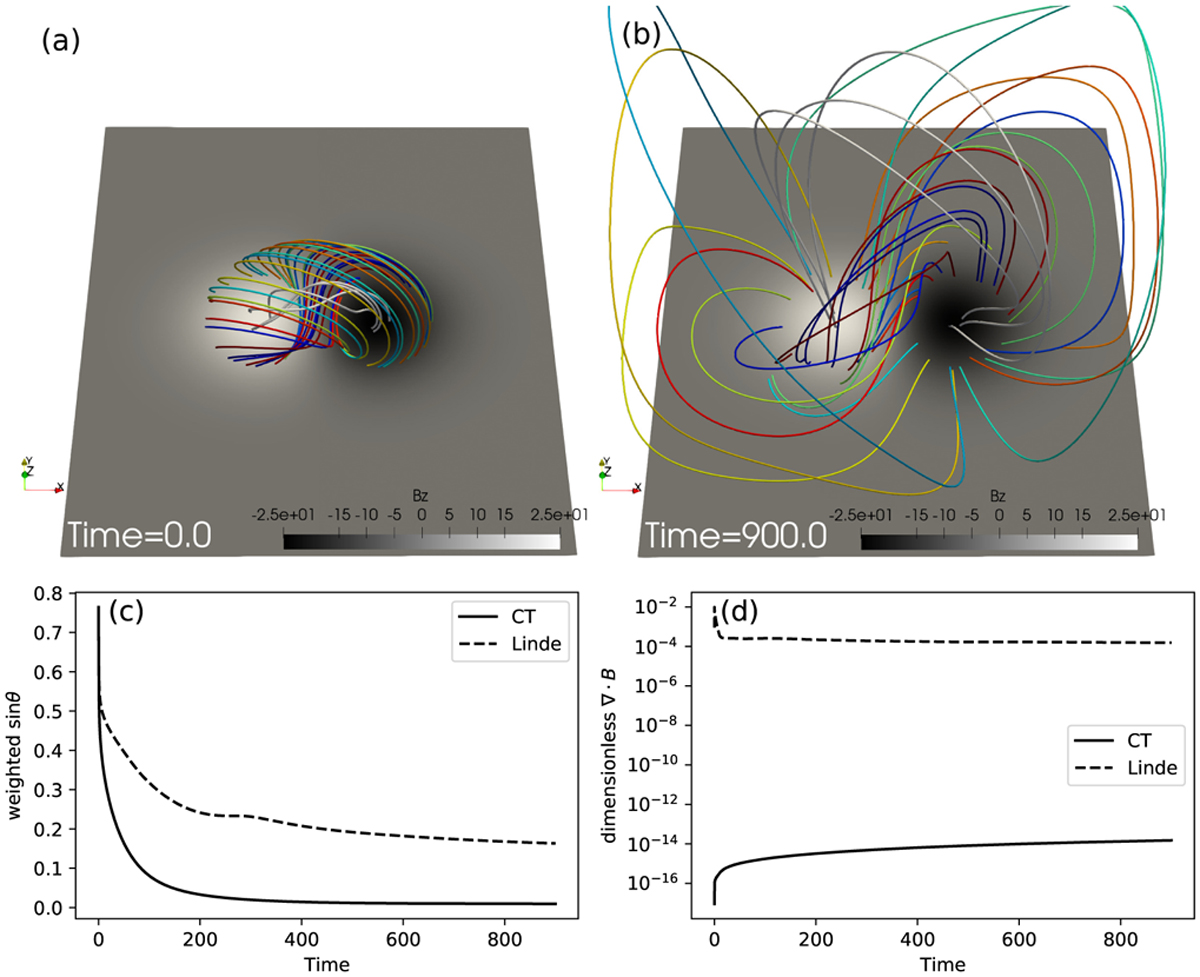 |
Fig. 13 MF relaxation of a non-force-free twisted magnetic flux tube. (a) Magnetic field lines of the flux tube in different colors at time 0. (b) Magnetic field lines starting from the same footpoints at time 900 of the ct run. (c) Degree of force-freeness as the weighted average of the sine of the angle between the magnetic field and the current density for the linde and ct run. (d) Degree of divergence-freeness as the average dimensionless divergence of the magnetic field for both runs. |
6.2 Inserting flux ropes using regularized Biot-Savart laws
Solar eruptive activities, such as flares and coronal mass ejections, are believed to be driven by the eruption of magnetic flux ropes. Many efforts have been devoted to model the magnetic field of such a configuration, such as the analytical Gibson-Low model (Gibson & Low 1998), Titov-Démoulin model (Titov & Démoulin 1999), and Titov-Démoulin modified model (Titov et al. 2014). Alternatively, nonlinear force-free field extrapolations are also applied to model flux ropes numerically (e.g., Canou et al. 2009; Guo et al. 2010). They use the vector magnetic field observed on the photosphere as the boundary condition, solve the force-free equation ∇ × B = αB, and derive the 3D coronal magnetic field. There are some drawbacks in these analytical and numerical methods. Most analytical solutions assume some geometric symmetries, such as a toroidal arc in the Titov-Démoulin model. On the other hand, many numerical techniques cannot derive flux rope structures in weak magnetic field region or when they detach from the photosphere, such as for intermediate or quiescent prominences. One way to alleviate this problem is to adopt the flux rope insertion method (van Ballegooijen 2004). However, this method uses an initial state far from equilibrium, which asks for many numerical iterations to relax and the final configuration is difficult to control.
Titov et al. (2018) proposed the RBSL method to overcome the aforementioned drawbacks. A force-free magnetic flux rope with an arbitrary axis path and an intrinsic internal equilibrium is embedded into a potential field. The external equilibrium could be achieved by a further numerical relaxation. The RBSL magnetic field, BFR, generated by a net current I and net flux F within a thin magnetic flux rope with a minor radius a(l) is expressed as
where AI(x) and AF(x) are the vector potentials, μ0 the vacuum permeability, C and C* the axis paths above and below the reference plane, KI(r) and KF(r) the integration kernels, R′ = dR/dl the unit tangential vector, l the arc length along the axis paths, and r ≡ r(l) = (x − R(l))/a(l). Titov et al. (2018) have provided the analytical forms of the integration kernels by assuming a straight force-free flux rope with a constant circular cross section. The axial electric current is distributed in a parabolic profile along the minor radius of the flux rope. With such analytical integration kernels, a flux rope with arbitrary path could be derived via Eqs. (42)–(44).
Guo et al. (2019) implemented the RBSL method in MPI-AMRVAC18. The module works for 3D Cartesian settings, allowing AMR. Figure 15 shows the magnetic flux rope constructed by the RBSL method overlaid on the 304 Å image observed by the Extreme Ultraviolet Imager (EUVI) on STEREO_B. In practice, one needs to determine four parameters to compute the RBSL flux rope, namely, the axis path C, minor radius a, magnetic flux F, and electric current density I. The axis path is determined by triangulation of stereoscopic observations of STEREO_A/EUVI, the Atmospheric Imaging Assembly (ΑΙΑ) on SDO, and STEREO_B/EUVI at 304 Å. The sub-photospheric counterpart C* is the mirror image of C to keep the normal magnetic field outside the flux rope unchanged. The minor radius is determined by half the width of the filament observed in 304 Å. The magnetic flux is then determined by the magnetic field observed by SDO/HMI at the footprints of the flux rope. Finally, the electric current  , where the sign is determined by the helicity sign of the flux rope.
With all these four parameters, the RBSL flux rope is computed via Eqs. (42)–(44). It has to be embedded into a potential magnetic field to construct a magnetic configuration conforming with magnetic field observations. When C* is the mirror image of C, the RBSL flux rope has zero normal magnetic field outside the flux rope, while the magnetic flux inside the flux rope is F. Therefore, we subtract the magnetic flux F inside the two footprints to compute the potential field. The RBSL flux rope field is embedded into this potential field. So, the normal magnetic field on the whole bottom boundary is left unchanged. The combined magnetic field might be out of equilibrium. We could relax this configuration by the MF method (Guo et al. 2016b,c). The final relaxed magnetic field is shown in Fig. 15. This magnetic field could serve as the initial condition for further MHD simulations.
The RBSL method can also be applied to construct the analytical Titov-Démoulin modified model. An example is presented in Guo et al. (2021), where the flux rope axis has to be a semicircular shape, and it is closed by a mirror semicircle under the photosphere. The major radius Rc is a free parameter. The flux rope axis is placed on the y = 0 plane and its center is located at (x, y) = (0,0). The minor radius a is also a free parameter. To guarantee the internal force-free condition, a has to be much smaller than Rc. Then, the flux rope has to be embedded into a potential field to guarantee the external force-free condition. The potential field is constructed by two fictional magnetic charges of strength q at a depth of dq under the photosphere, which are along the y-axis at y = ±Lq. The electric current and magnetic flux are determined by Eqs. (7) and (10) in Titov et al. (2014).
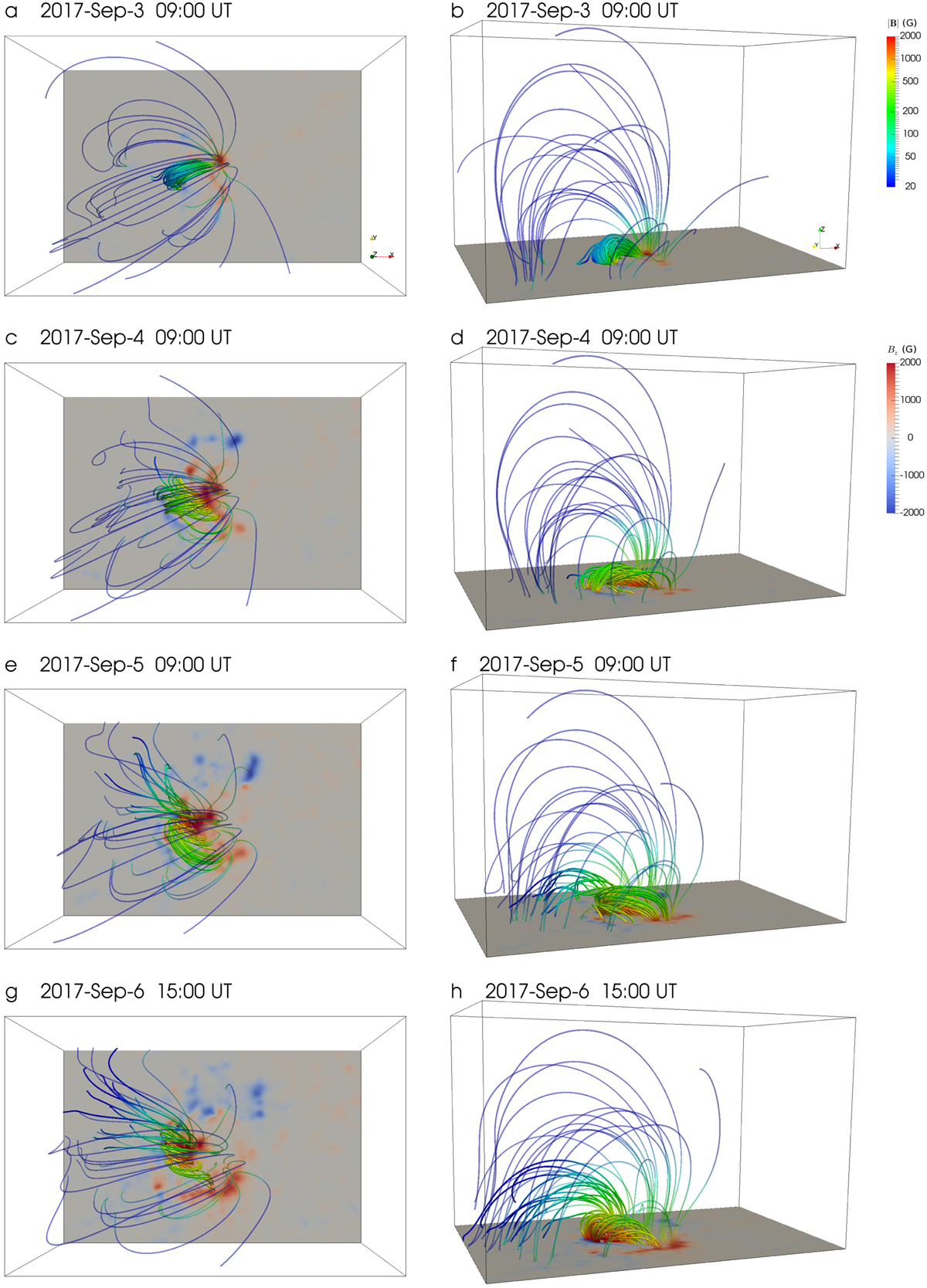 |
Fig. 14 Evolution of magnetic field lines in the data-driven time-dependent MF simulation. The left column shows a top view, and the right column shows a side view. The slice on the bottom displays the normal magnetic field, Bz. The magnetic field lines are colored according to the field strength. |
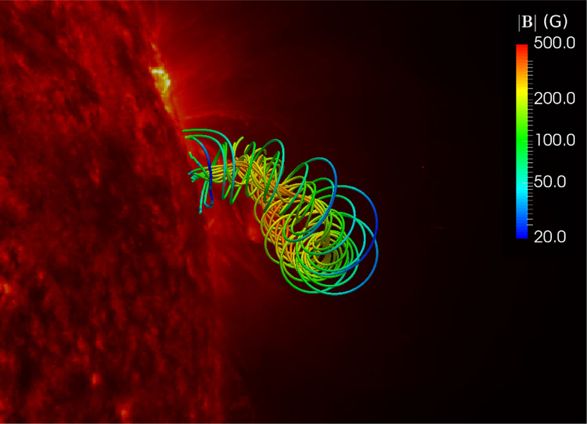 |
Fig. 15 Magnetic flux rope constructed via RBSL overlaid on the STEREO_B/EUVI 304 Å image observed at 01:11 UT on 2011 June 11. |
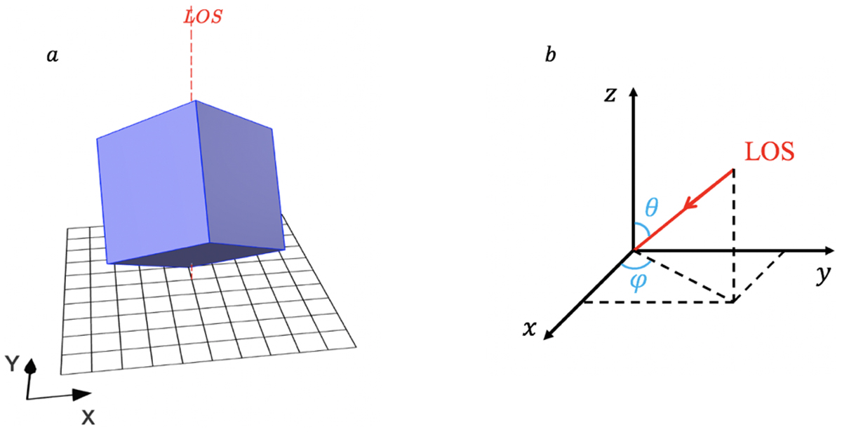 |
Fig. 16 Ingredients for the (on-the-fly or post-process) synthetic imaging, (a) Simulation box (blue cube), LOS (dashed red line), and EUV image plane (black mesh). The EUV image plane is perpendicular to the LOS. (b) LOS depends on θ and φ at simulation box coordinates. |
6.3 Synthetic observations
For solar applications, it is customary to produce synthetic views on 3D simulation data, and various community tools have been developed specifically for post-processing 3D MHD data cubes. For example, the FoMo code (Van Doorsselaere et al. 2016) was originally designed to produce optically thin coronal EUV images based on density, temperature and velocity data, using CHIANTI (see Del Zanna et al. 2021 and references therein) to quantify emissivities. FoMo includes a more complete coverage of radio emission of up to optically thick regimes, and Pant & Van Doorsselaere (2020) provide a recent example of combined MPI-AMRVAC-FoMo usage addressing nonthermal linewidths related to MHD waves. Another toolkit called FORWARD (Gibson et al. 2016) includes the possibility to synthesize coronal magnetometry, but is Idl-based (requiring software licenses) and an implementation for AMR grid structures is as yet lacking.
Since synthetic data for especially optically thin coronal emission is key for validation purposes, we now provide modules that directly perform the needed ray-tracing on AMR data cubes, in src/physics/mod_thermal_emission.t. The module contains temperature tables specific for ΑΙΑ, IRIS and EIS instruments, with coverage for various wavebands. One can synthesize both EUV and soft X-ray emission, and the module can be used for synthetic images or for spectral quantifications. Images in vti format are readily produced either during runtime or in a post-processing step, where the user controls the relative orientation of the line of sight (LOS) to the data cube. We use this for 3D Cartesian data sets from MHD, allowing AMR.
As the first step in synthesizing an EUV image, a 2D table is created to record the luminosity of each image pixel. We assume that an EUV image has uniform pixel size; for example, the pixel size of SDO/ΑΙΑ images is 0.6 arcsec (Lemen et al. 2012). The spatial link between the EUV image plane and the 3D simulation box refers to Fig. 16a, where the mapping between simulation box coordinates (x, y,z) and EUV image coordinates (X, Y) is accomplished using the unit direction vectors XI and YI of the image plane at simulation coordinates:
The vectors XI and YI are both perpendicular to the LOS and to each other, and are given by
where VLOS is the LOS vector in simulation box coordinates. VLOS can be written as
with the user-given parameters θ and φ (Fig. 16b). The user-defined parameter (x0,y0,z0), which has a default value of (0, 0, 0), can be any point in the simulation box and can then be mapped to the EUV image coordinate origin (X = 0, Y = 0).
The integral EUV flux from each cell in the simulation box is computed and then distributed over the table, where the cell flux is given by
where Nec is the cell electron number density, Tec is the cell electron temperature, G is the contribution function of the corresponding EUV line given by the CHIANTI atomic database, and Δx, Δy, and Δz are the cell sizes in three directions (Del Zanna et al. 2021). Due to instrument scattering, a single point source will appear as a blob in EUV observations. This effect is taken into consideration when distributing cell flux to image pixels by multiplying a Gaussian-type point spread function (PSF; Grigis et al. 2013). The resulting pixel
flux is given by
where i is the cell index, Ic,i is the integral EUV flux from the ith cell, (Xc,i, Yc,i) is the mapping result of the cell center at the image plane, and Xmin, Xmax, Ymin and Ymax give the borders of the pixel. The standard deviation σ of the PSF is taken from the related papers of the corresponding spacecraft, and is usually close to the pixel size. When the cell size is not small enough compared to the EUV image pixel size (for example, the projection of any cell edge at the image plane is larger than half the pixel size), a cell is split into multiple parts before the calculation of Eqs. (50)–(52) in order to improve the integral accuracy.
Figure 17 shows a snapshot of a data-driven MHD model for the X1.0 flare at 15:35 UT on 2021 October 28. The 3D MHD model considers a full energy equation with background heating, thermal conduction, and optically thin radiation losses. A detailed analysis of this simulation will be presented in a future paper. Here, we use a single snapshot from the evolution to synthesize EUV images, to demonstrate this new capability of MPI-AMRVAC. Figure 18 shows comparisons of SDO/AIA observations and the synthesized EUV images from the data-driven MHD model. We select three different wavebands at 94 Å, 171 Å, and 304 Å. It is found that the simulation and its synthesized EUV images reproduces qualitatively various aspects seen in the flare ribbons. In contrast to the actual observed images, coronal loops are not reproduced very accurately (as shown in Figs. 18c,d), and the simulation displays a relatively strong spherical shock front, seen in all three wavebands. These aspects rather call for further improvement of the (now approximate) radiative aspects incorporated in the data-driven MHD model, but these can still be improved by adjusting the heating-cooling prescriptions and the magnetic field strength. Here, we only intend to show the synthesizing ability of MPI-AMRVAC, which has been clearly demonstrated.
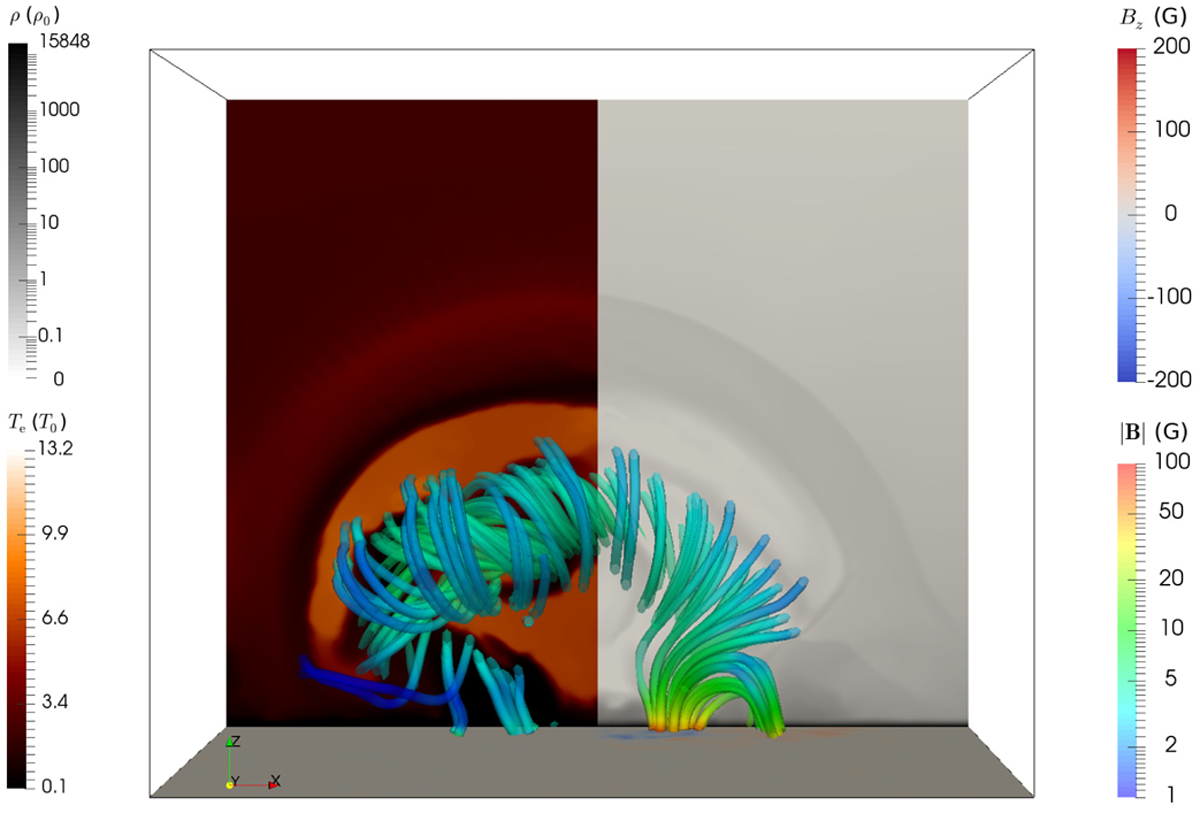 |
Fig. 17 Data-driven MHD model, with all energetics incorporated. The vertical slices show the temperature on the left and density on the right. The magnetic field lines are colored according to the field strength. The bottom slice displays the normal magnetic field, Bz. |
7 Handling particles and field lines
7.1 Sampling, tracking, or Lorentz dynamics
The src/particle folder contains all options for handling “particle” dynamics that one may relate to the PDE system at hand. For any of the PDE modules listed in Table 1, computational particles can be employed to meaningfully sample all solution values at pre-chosen fixed or dynamically evolving locations. We illustrate this with a 2D linear scalar advection problem, where the particle module samples the solution at three distinct locations: one fixed in space and time, another one moving with constant speed on a vertical straight line, and a third location that follows a uniform circular motion. On a square domain, the diagonally advected profile corresponds to our VAC logo, with constant values ρ = 0.5 exterior, and ρ = 2 interior to the letters, and Fig. 19 shows the ρ(x, y, t = 1) distribution for a 4-level AMR run using a three-step TVDLF run with the koren limiter (Koren 1993). The sampling “particles” and their trajectories are shown in blue. The plots on the right show the sampled data for the three particles as a function of time. The complete setup19 demonstrates how the user can add and define additional variables (here corresponding to the exact solution ρexact(x, y, t) at given time t and the error with respect to the exact solution) and how to add a pay-load (namely the sampled exact solution) to the particle sampler. This kind of sampling on prescribed user-defined trajectories could be relevant for 3D space-weather-related MHD simulations as done by ICARUS (Verbeke et al. 2022), for comparison with actual spacecraft data. The interpolations from (AMR) grid cell centers to locally sampled data are done by linear (bilinear in 2D or trilinear in 3D) interpolation, where also linear interpolation in time is performed when dynamic evolutions occur. The actual subroutine for interpolating any field variable to a specific grid location can be modified at will, and is called interpolate_var in the particle/mod_particle_base.t module. Other interpolation schemes (e.g., quadratic or higherorder) can be implemented there.
A second use-case for the src/particle folder is specific to any PDE system featuring a vector velocity field, such as the HD or MHD systems. In that case, we may be interested in gas or plasma properties at locations that follow the flow, and hence positions that are merely advected in a Lagrangian fashion. This is possible with the mod_particle_advect.t module.
Whenever plasma is involved, such as in an MHD (or two-fluid plasma-neutral) setting, we can also quantify instantaneous magnetic and electric field data from the MHD variables. This can then be used to compute the trajectories of charged test particles with a given mass, m, and charge, q, according to the standard Lorentz equation, where acceleration a follows from ma = q (E + v × B) or from its fully relativistic variant (see, e.g., Ripperda et al. 2018). The latter was used in Zhao et al. (2021) to analyze relativistic particle acceleration processes in 2D resistive MHD simulations of chaotic island formation (also occurring in the tilt evolution from Sect. 4.2.2). We demonstrate here the capability of tracing charged particles in MHD simulations by using the electromagnetic field data from Sect. 4.2.2 at t = 8.5 (roughly corresponding to Fig. 9) and evolving particles in this fixed MHD background. Figure 20 (top left) shows the trajectories of selected particles (evolved foratime t = 0.5)in the central xy region [−0.25, 0.25] × [−0.125, 0.125] of the aforementioned MHD run, where island interaction creates chaotic magnetic structures and strong out-of-plane currents Jz. The same figure (top right, bottom left, bottom right) presents a zoom-in onto three selected particle trajectories, showing explicitly the oscillatory and drift motion of charged particles around and across magnetic field lines. Several integration methods are available to numerically solve charged-particle motion in MPI-AMRVAC, either in the Newtonian or in the relativistic limit.
In many astrophysically relevant situations, one may be faced with unusually large differences in the (small) length scale set by the charged particle local gyroradius, and the one associated with (gradients in) the background electromagnetic field quantities. In that case, it can be advantageous to work with the guiding center approximation (GCA) where one solves a set of ordinary differential equations where the fast gyro-motion is averaged out. The use of GCA equations in MPI-AMRVAC was, forexample, demonstrated in 3D MHD setups of KH unstable magnetopause setups featuring particle trapping in Leroy et al. (2019). The various options for the relativistic Lorentz equation integrators implemented in MPI-AMRVAC, as well as the governing GCA equations with references to their original sources can be found in Ripperda et al. (2018). A summary in the online documentation is the markup-document in doc/particle.md.
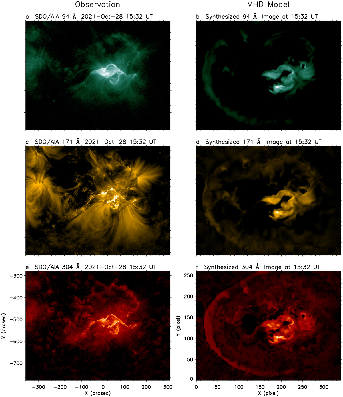 |
Fig. 18 Comparison between SDO/AIA observations and synthesized EUV images from a data-driven MHD model (as in Fig. 17), including a full energy treatment. The left column shows the SDO/AIA observations at wavebands of (a) 94 Å, (c) 171 Å, and (e) 304 Å. The right column shows the emission at the same waveband as the left synthesized from the MHD model at the same time. |
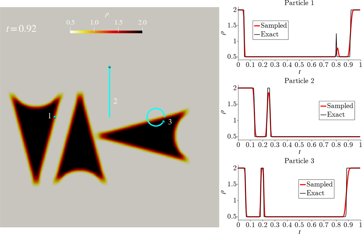 |
Fig. 19 Demonstration of the sampling possibilities, where a 2D scalar linear advection problem is augmented with sampled solutions at three locations that follow user-specified orbits. The left panel shows the solution at t = 0.92, along with the trajectories of sampling particles (blue spheres and lines). The right panels show the numerical (in red) and the analytic solution (black) as a function of time for the three locations. An animation is provided online. |
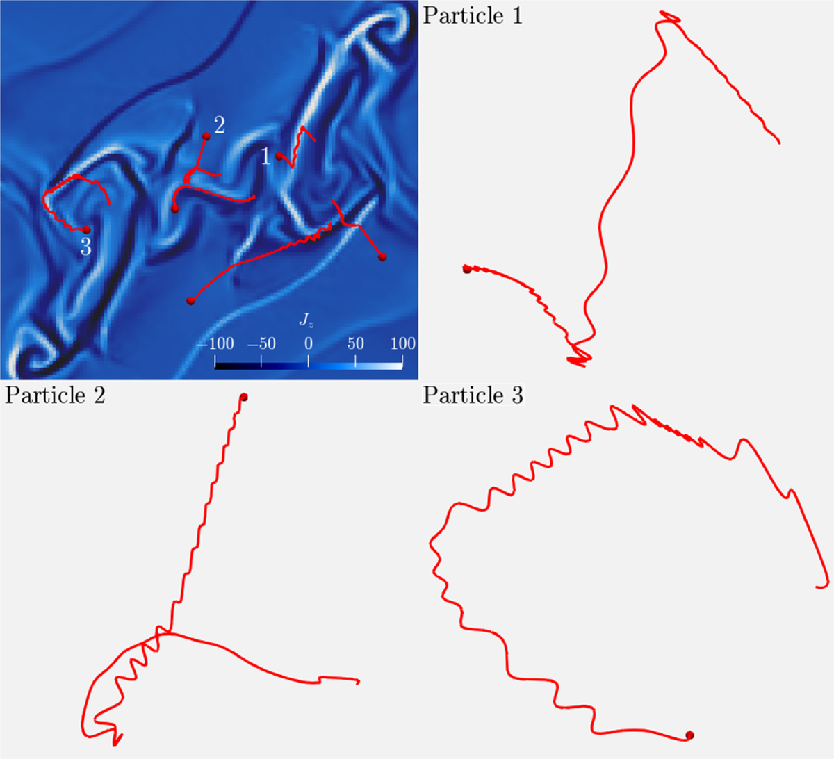 |
Fig. 20 Demonstration of charged-particle tracing in an MHD simulation. The background fluid state is taken from Sect. 4.2.2 and kept fixed while several charged particles are traced (red lines in the top-left panel) by numerically solving the equations of motion. Selected zoomed-in trajectories (top-right, bottom-left, and bottom-right panels) show the typical oscillatory and drift motion of charged particles around and across magnetic field lines. An animation is provided online. |
7.2 Field line tracing
We introduce a generic field line tracing module (in src/module/mod_trace_field.t, which is able to trace various types of field lines that start at user-specified points, either during runtime or in post-processing fashion. At the moment, this functionality works for 3D Cartesian AMR grids (but does not account for possibly stretched grids discussed in Sect. 8.3). The flow chart for tracing a single magnetic field line through a memory-distributed block-AMR setting has been introduced in Ruan et al. (2020; their, Fig. B1). We now add a functionality to trace multiple field lines in parallel, where now multiple starting points can be provided for a set of field lines to be traced through the AMR grid hierarchy. We also generalize the implementation to handle any type of vector field, such that we can plot or trace (1) magnetic field lines in MHD (or multi-fluid) settings, but also (2) flow streamlines for the velocity field, and (3) any user-defined vector field (e.g., useful for visualizing or quantifying electric fields and currents). This functionality is demonstrated in Fig. 3 where it is used to compute and visualize velocity streamlines, and in Fig. 9 where the magnetic field lines shown are also calculated with this module. For these 2D cases (the tracing implementation works in 2D and 3D), we employ the method presented in Jobard & Lefer (1997) to select seed points to get evenly spaced streamlines or field lines.
During this tracing, users can ask to interpolate any set of self-defined derived quantities to the field lines. This ability is, for example, crucial to the TRAC method for handling sharp transitions in temperature and density fields, where along the trajectories of magnetic field lines, the temperature gradients along the line tangent direction are required (Zhou et al. 2021). In Ruan et al. (2020), magnetic field lines in a 2D reconnection setup inspired by the “standard solar flare model” were computed during runtime, and model equations along the field lines were solved to quantify how the energy release by reconnection gets dynamically deposited in remote locations (by energetic electron beams that collide with lower-lying, denser chromosphere material). This involves back and forth interpolations between grid and field lines. Together with the general functionality provided through the particle module (Sect. 7.1), it then becomes possible to provide dynamically evolving seed points such that one traces the exact same field lines, simply by using Eulerian advection on the seeds.
8 Data processing and technical aspects
8.1 Customized user interfaces
For any new application, the minimal requirement is to code up an application-specific mod_usr.t file where at least the initial condition for all involved variables must be provided. The input parameter file amrvac.par makes use of Fortran name lists to then select the time stepping scheme, the spatial discretization, I/O aspects, boundary conditions, and parameters that control the evolving AMR grid structure. For every PDE system from Table 1, equation-specific parameters may need to be set as well.
The actual code versatility follows from the many ways to allow user-customized adaptations. These include as most commonly used ones:
- the addition of specific source terms in the equations, and their corresponding effect on time step constraints for explicit time stepping strategies;
- the definition of user- or application-specific (de)refinement strategies, based on combinations of either purely geometric or solution-derived quantities;
- the design of specific boundary conditions on user-selected variables;
- the way to add derived variables to the I/O routines or to carry out post-processing during conversion or runtime on data files;
- the possibility to process data at every timestep;
- the way to handle particle data and payloads.
The complete list of all customized subroutine interfaces is given in src/mod_usr_methods.t. Many examples of their intended usage can be found in the tests folder.
8.2 Initializing from datacubes or driving boundaries
The code offers various possibilities to read in structured data sets, which can be used for initialization or boundary driving purposes. For example, the Alfvén shock test in Sect. 4.2.1 shows how a vtk image can be used to set the density at time t = 0 in some part of the domain, while 2D and 3D advection tests can use the same image as a boundary condition. An impression of such 2D boundary-driven advection using the alfven.vtk image20, while enforcing user-controlled, purely geometric AMR (only a central region is at the highest AMR level) is provided in Fig. 21. Such 2D advection of the image mimics a faxing process where the image gets advected into the domain as time proceeds (this is a time-dependent 1D boundary driving realized by a single 2D image), and 3D variants would realize time-dependent 2D boundary driving. Initializing data uses the src/mod_init_datafromfile.t module, which currently expects a vtk formatted data set (2D or 3D). This can easily be adjusted to read in structured data from other simulation codes, for detailed inter-comparisons, or for revisiting structured grid data evolutions with AMR runs that may zoom in on details. All functionality discussed above stores the read-in data in a lookup-table, which allows for easy and efficient interpolations to the AMR grid. As usual, when reading in external data, the user must beware of a possible need to introduce floor values (e.g., ensuring positive densities and/or pressures), or handling data outside the region covered by the given dat-acube. The time-dependent MF module discussed in Sect. 6.1 is yet another example of how one can handle time-dependent boundary data, as provided from external files.
8.3 AMR and multidimensional stretching in orthogonal coordinates
MPI-AMRVAC allows for anisotropic grid stretching, that is, independent grid stretching prescriptions for each spatial coordinate, combined with AMR, for any geometry. A “stretched” grid does not imply enlarging the domain, but rather the use of nonuniform grid cells to cover a given domain, with cells that become gradually larger (or smaller) in a stretched direction. This generalizes our previously documented purely radial grid stretching for spherical (or polar/cylindrical) applications as documented in Xia et al. (2018). Currently two stretching configurations are supported, namely: (1) unidirectional stretching, where every cell is stretched by a constant factor (the “stretching factor”) in the specified spatial direction from cell to cell; (2) symmetric stretching, where one can specify the amount of blocks that should remain uniform, with the remaining blocks on either side stretched. This must have an even number of grid blocks on the base AMR level, and adopts a central symmetry.
Figure 22 showcases this capability for 3D cylindrical (left panel) and spherical (right panel) geometries. In both examples a uniform medium has been set up in which denser, uniform spheres have been added to the domain to trigger AMR. The domain itself consists of a 603 grid with six blocks in each direction. The cylindrical case employs unidirectional radial stretching with a stretching factor of 1.05, combined with symmetric stretching for all 6 blocks in the z-direction (so no uniform central blocks along the z-axis). The spherical case on the other hand employs anisotropic stretching in all three directions, r is unidirectionally stretched with stretching factor of 1.02. Both the θ– and φ directions are symmetrically stretched in four blocks with stretching factors of 1.15 and 1.2, respectively. We note that these factors have been exaggerated for visual effects, in typical use cases a stretching factor between 1.01 and 1.05 is reasonable.
We caution that not all reconstruction procedures to compute the cell edge from cell center values are fully compatible with this stretching, but, for example, the WENO flavors listed in Table 4 with the “nm” extension can all be used reliably. These have been introduced as the nonuniform modified WENO variants in Huang et al. (2018).
 |
Fig. 21 Density from a 2D, boundary-driven advection problem: the alfven.vtk image is used to set time-dependent boundary values at the top edge, advected into the domain by a constant advection speed, v = −ey. We show the solution at t = 1.15 on a [0,1] × [0, 1.5] domain. The four-level AMR hierarchy is purely geometrically controlled in this example, forcing the central band of the image to appear sharpest. |
8.4 Bootstrapping: Handling small thermodynamic quantities
Whenever extreme contrasts occur in thermodynamic (densities, pressures, temperatures) or magneto-kinetic quantities (high or low plasma beta and/or Mach numbers) within the simulated domain, it may become crucial to impose bootstrapping strategies to prevent unphysical states (negative pressure, or too low densities) from ever occurring. In the typical finite-volume methods as used here (and in many other software frameworks), this can be enforced numerically in a variety of ways. MPI-AMRVAC imposes such strategies by the global logical parameters check_small_values and fix_small_values, which by default are .true. and .false.. This default strategy means that a simulation will stop and simply report the error. This may signal user (or developer) implementation errors, which must be dealt with first. It may also signal problems in boundary treatments, or relate to as yet unresolved initial or instantaneous variations that may need higher resolutions. Having many choices of schemes and limiters then comes in handy, since when problems persist for the most robust or diffusive combinations, a bug is almost surely at play.
However, there may be (rare) situations where roundoff errors, or the various intricate nonlinear prescriptions (such as involved in limited reconstructions) themselves create unphysical conditions, for example when recently updated conserved variables no longer translate to physical primitive variables. Therefore, we allow for activating fixes controlled by small_pressure and small_density user inputs, and offer a number of ways to recover from unphysical states. In practice, these bootstrapping procedures are then in effect on entry for the step translating conservative to primitive variables, can be used when switching total to partial energy density contributions, and could enforce a thermal pressure calculation to always return values equal to or above small_pressure. Fixes could also be enforced at the end of specific source term additions, but the bootstrapping will never modify magnetic fields, and will obviously no longer strictly obey energy conservation (or mass conservation when having positive small_density). It is then advised to monitor this possible accumulation of errors. Such bootstrapping was also found necessary to handle the occurring near-vacuum regions in thermal runaway simulations (as in Sect. 4.1.3) in an MHD setting (Hermans & Keppens 2021). Bootstrapping measures may simply replace faulty values by the user-set small_pressure and small_density combinations, or work with a user-controlled area (line, square or cube in 1D, 2D, or 3D) around the problem cell, to perform averaging from surrounding non-problematic cells on the primitive entries. In combination with specific checks enforced on the reconstructions from cell center to cell edges, this bootstrapping should then avoid fatal code crashes, without sacrificing physical reality. It is to be noted that various codes handle this in undocumented fashion, and may exploit (excessive) hyperdiffusion or parameter-rich clipping strategies whenever strong shocks, unresolved gradients, or actual discontinuities are at play.
8.5 Data analysis routines and visualizations
Natively, MPI-AMRVAC outputs its data in a custom data format (hereafter referred to as “data files” after its use of the typical .dat extension), which relies on standard I/O routines. This allows for optimized read/write I/O operations, thereby minimizing the amount of time needed to write data to disk. The custom (and compact) data file format also implies efficient reading of the data, which the code can use to restart and/or continue the simulation from a previous snapshot. One major drawback of storing data this way is that a custom data format as employed here is unrecognizable by third-party software used for analysis or visualization. To mitigate this issue the code has various conversion routines implemented, which can convert existing data files to more standardized formats such as .vtu (VTK unstructured data) that are directly accessible by visualization packages such as ParaView or VisIt. While this approach is reasonable for smaller simulations it raises various issues for large-scale runs that output huge data files. The need for .vtu files for example results in additional usage of disk space and more I/O-time due to converting. Furthermore, data files from large simulations are usually too big to load directly in memory.
For large data sets users can make use of yt, an open-source Python package for data analysis and visualization tailored to astrophysical codes (Turk et al. 2011). Yt’s core functionality is written in Cython and heavily relies on NumPy (and its C-API) for fast and efficient array operations. We developed a dedicated frontend that ensures yt can directly load native MPI-AMRVAC data files, eliminating the need for conversion to other data formats. Additionally, data loading through yt makes use of memory-mapping, where a first pass over the data maps the on-disk structure to physical space prior to actually loading. Data are then selectively retrieved based on queries by the user, which avoids caching all data directly into memory. All of MPI-AMRVAC’s possible geometries are supported as well. Some features such as staggered or stretched grids and magnetic field splitting, amongst others, are not yet supported, but will be in due time.
Historically, MPI-AMRVAC only saves the conserved variables to the datfile, but the corresponding .vtu files may switch to primitive variables, or even add any number of user-added additional fields (such as temperature, divergence of the velocity, etc.). Similarly, user-defined fields can be saved in data files21, which can later be loaded in yt. Of course, adding more variables implies even more disk space. To mitigate this, the user has full control on how many (and which) derived variables are stored to the .vtu and .dat files, and can generate these post-process. A major advantage yt has over third-party visualization tools is the use of so-called derived fields. These are quantities that are derived from one or more primitive variables and can be defined by the user. These fields are then composed using the queried data and allows visualization of (most) quantities that can be derived from others without having to save them to disk.
It should be noted that the use of ParaView or VisIt versus yt is application-dependent and should be regarded as complementary. For smaller data sets users may prefer the graphical user interface of third-party software for visualization rather than Python code. For large data sets yt is (or should be) preferred.
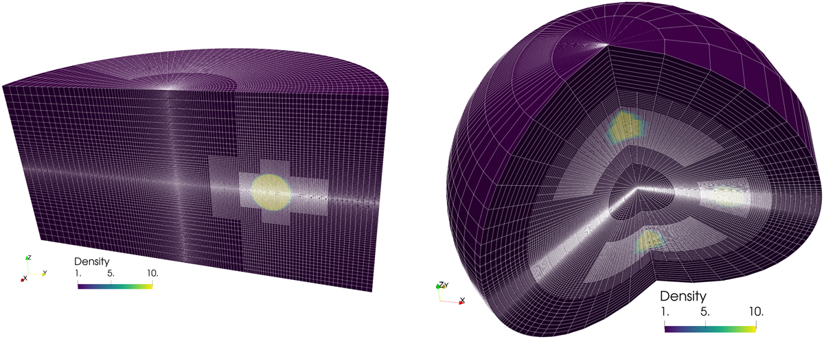 |
Fig. 22 Anisotropic grid stretching for cylindrical or spherical runs. In a 3D cylindrical (left) and spherical (right) AMR grid, both cases are unidirectionally stretched in the radial direction, with additional symmetric z-stretching for the cylindrical one and both θ and ϕ symmetric stretching for the spherical one. |
9 Future directions
We have provided an updated account of the open-source MPI-AMRVAC 3.0 framework, one among many AMR-supporting frameworks in active use for computational solar and astrophysically motivated research. We close this paper with an outlook on further promising developments.
Most of the currently implemented physics modules (HD, MHD, plasma-neutral two-fluid) assume no or purely local interactions (adequate for optically thin conditions) between the gas or plasma and the radiation field. The radiative-hydro module (Moens et al. 2022) that uses FLD, now included in the 3.0 version, realizes only the first step toward more consistent radiative (M)HD treatments. First intrinsically coupled radiative-MHD modeling with MPI-AMRVAC includes 2D axisymmetric magnetized wind studies for hot stars (Driessen et al. 2021), where line driving is essential both for the wind generation and for realizing conditions prone to the line-deshadowing instability, causing clumpy, magnetized trans-magnetosonic winds. These models use an isothermal closure relation but handle the line-driven aspect of hot, massive star winds by means of a cumulative force contribution22, as introduced by Castor et al. (1975).
The FLD formulation can easily be carried over to an MHD setting, while both HD and MHD formulations can also exploit first-moment M1 closure formulations, as realized in, for example, RAMSES-RT (Rosdahl & Teyssier 2015). Both FLD and M1 radiative-(M)HD formulations have the distinct advantage that they in essence translate to fully hyperbolic PDE systems (with source term couplings), and this is readily adjustable to any framework, such as MPI-AMRVAC. Of course, in solar physics contexts, current state-of-the-art (non-AMR) codes such as Stagger (as used in Stein & Nordlund 2006), Bifrost (Gudiksen et al. 2011; Nóbrega-Siverio et al. 2020), MURaM (Vögler et al. 2005), MANCHA3D (Khomenko et al. 2018; Navarro et al. 2022), RAMENS (Iijima & Yokoyama 2017), and CO5BOLD (Freytag et al. 2012) focus on 3D radiative-MHD simulations that include magneto-convection in optically thick sub-photospheric layers, use optically thin prescriptions for the corona, and have a more sophisticated treatment of the radiative effects known to be important in solar chromospheric layers. This includes handling partial ionization effects through MHD with ambipolar diffusion or two-fluid plasma-neutral modeling, as implemented in MPI-AMRVAC 3.0 (Popescu Braileanu & Keppens 2021, 2022). However, they are especially concerned with more advanced radiative transfer aspects, going beyond local thermo-dynamic equilibrium and approximating the complex chromo-spheric radiative aspects, as realized recently within MURaM, for example by Przybylski et al. (2022). Future efforts toward such truly realistic radiative-MHD or radiative-multi-fluid models on evolving, block-AMR settings are highly desirable.
MPI-AMRVAC 3.0 still uses standard Fortran with MPI for parallelization purposes (described in Keppens et al. 2012), and our suite of automated tests includes compiling the code in 1D to 3D setups with various versions of gfortran or Intel compilers. The code can use hybrid OpenMP-MPI parallelism, where the OpenMP pragmas ensure thread-based parallelism over the blocks available within a shared memory. The related BHAC code considerably improved on this hybrid parallelization aspect (Cielo et al. 2022). For truly extreme resolution simulations, one needs further code restructuring (especially the internal boundary exchange involved with AMR meshes) toward task-based parallelism. To optimally exploit the modern mixed CPU-GPU platforms, we plan to explore OpenACC23 or the possibilities for GPU off-loading provided by OpenMP. Similar modern restructuring efforts of Athena++ to K-Athena to make efficient usage of tens of thousands of GPUs are documented in Grete et al. (2021).
Even when none or only approximate radiative effects are incorporated in our 2D or 3D (M)HD settings, one can use dedicated radiative transfer codes to assess the model appearance in synthetic views. For infrared views of stellar winds colliding with dust production zones in Hendrix et al. (2016), this was handled by post-processing, where the native MPI-AMRVAC data files were inputs to SKIRT (Camps & Baes 2015). A similar coupling of MPI-AMRVAC to the recent MAGRITTE radiative transfer solver is presented in De Ceuster et al. (2020). For solar physics applications, ongoing research is using the Lightweaver (Osborne & Milic 2021) framework to synthesize spectral information from the latest prominence formation models (Jenkins & Keppens 2022).
To ultimately do justice to plasma physics processes that are intrinsically multi-scale, we may need to go beyond pure fluid treatments. This is the main reason for developing visionary frameworks such as DISPATCH (Nordlund et al. 2018) and PATCHWORK (Shiokawa et al. 2018). They envision hierarchically coupled physics and grid-adaptive aspects, which still pose various technical algorithmic challenges. First steps toward such coupled particle-in-cell-MHD efforts in MPI-AMRVAC contexts have been explored in Makwana et al. (2017, 2018). Complementary hybrid particle-MHD modeling has been realized in van Marle et al. (2018), in a 2D3V setting applied to particle acceleration processes at MHD shocks, following earlier approaches from Bai et al. (2015). This functionality is currently not included in the MPI-AMRVAC 3.0 release, since we prioritized a basic restructuring of the particle and field tracing modules, as documented here. We note that the development part of the code can be inspected online24, and the corresponding new branches can be followed on GitHub. Test particle studies may in the future benefit from the need for hybrid particle pushers (Bacchini et al. 2020), in which automated switching between GCA and Lorentz treatments has been demonstrated. The open-source strategy followed implies that many more research directions can be pursued, and we welcome any addition to the framework.
Acknowledgements
We thank the referee for constructive comments and suggestions. Y.Z. acknowledges funding from Research Foundation – Flanders FWO under the project number 1256423N. B.P. acknowledges funding from Research Foundation – Flanders FWO under the project number 1232122N. F.B. acknowledges support from the FED-tWIN programme (profile Prf-2020-004, project “ENERGY”) issued by BELSPO. C.X. acknowledges funding from the Basic Research Program of Yunnan Province (202001AW070011), the National Natural Science Foundation of China (12073022). Y.G. is supported by the National Key Research and Development Program of China (2020YFC2201201) and NSFC (11773016 and 11961131002). This project received funding from the European Research Council (ERC) under the European Union’s Horizon 2020 research and innovation program (grant agreement No. 833251 PROMINENT ERC-ADG 2018). Further, this research is supported by Internal funds KU Leuven, project C14/19/089 TRACESpace and FWO project G0B4521N. Visualisations used the open source software ParaView (https://www.paraview.org/), Python (https://www.python.org/) and yt (https://yt-project.org/). Resources and services used in this work were provided by the VSC (Flemish Supercomputer Center), funded by the Research Foundation – Flanders (FWO) and the Flemish Government. We acknowledge code contributions by masterstu-dents Robbe D’Hondt and Brecht Geutjens, by Dr. Jannis Teunissen, Dr. Florian Driessen, and Dr. Clément Robert, and by PhD candidates Veronika Jerčić, Joris Hermans, and Nicolas Moens.
References
- Acker, F., B. de R. Borges, R., & Costa, B. 2016, J. Comput. Phys., 313, 726 [NASA ADS] [CrossRef] [Google Scholar]
- Alexiades, V., Amiez, G., & Gremaud, P.-A. 1996, Commun. Numer. Methods Eng., 12, 31 [Google Scholar]
- Aràndiga, F., Martí, M. C., & Mulet, P. 2014, J. Sci. Comput., 60, 641 [CrossRef] [Google Scholar]
- Ascher, U. M., Ruuth, S. J., & Spiteri, R. J. 1997, Appl. Numer. Math., 25, 151 [CrossRef] [MathSciNet] [Google Scholar]
- Bacchini, F., Ripperda, B., Porth, O., & Sironi, L. 2019, ApJS, 240, 40 [Google Scholar]
- Bacchini, F., Ripperda, B., Philippov, A. A., & Parfrey, K. 2020, ApJS, 251, 10 [NASA ADS] [CrossRef] [Google Scholar]
- Bai, X., Caprioli, D., Sironi, L., & Spitkovsky, A. 2015, ApJ, 809, 55 [NASA ADS] [CrossRef] [Google Scholar]
- Balsara, D. S., & Shu, C.-W. 2000, J. Comput. Phys., 160, 405 [NASA ADS] [CrossRef] [Google Scholar]
- Balsara, D. S., & Spicer, D. S. 1999, J. Comput. Phys., 149, 270 [NASA ADS] [CrossRef] [Google Scholar]
- Berger, M. J., & Colella, P. 1989, J. Comput. Phys., 82, 64 [CrossRef] [Google Scholar]
- Borges, R., Carmona, M., Costa, B., & Don, W. S. 2008, J. Comput. Phys., 227, 3191 [NASA ADS] [CrossRef] [Google Scholar]
- Brackbill, J. U., & Barnes, D. C. 1980, J. Comput. Phys., 35, 426 [NASA ADS] [CrossRef] [Google Scholar]
- Braginskii, S. I. 1965, Rev. Plasma Phys., 1, 205 [Google Scholar]
- Bryan, G. L., Norman, M. L., O’Shea, B. W., et al. 2014, ApJS, 211, 19 [Google Scholar]
- Čiada, M., & Torrilhon, M. 2009, J. Comput. Phys., 228, 4118 [CrossRef] [Google Scholar]
- Camps, P., & Baes, M. 2015, Astron. Comput., 9, 20 [Google Scholar]
- Canou, A., Amari, T., Bommier, V., et al. 2009, ApJ, 693, L27 [NASA ADS] [CrossRef] [Google Scholar]
- Castor, J. I., Abbott, D. C., & Klein, R. I. 1975, ApJ, 195, 157 [Google Scholar]
- Cavaglieri, D., & Bewley, T. 2015, J. Comput. Phys., 286, 172 [NASA ADS] [CrossRef] [Google Scholar]
- Cheong, P. C.-K., Lam, A. T.-L., Ng, H. H.-Y., & Li, T. G. F. 2021, MNRAS, 508, 2279 [NASA ADS] [CrossRef] [Google Scholar]
- Cheong, P. C.-K., Pong, D. Y. T., Yip, A. K. L., & Li, T. G. F. 2022, ApJS, 261, 22 [NASA ADS] [CrossRef] [Google Scholar]
- Cheung, M. C. M., & DeRosa, M. L. 2012, ApJ, 757, 147 [NASA ADS] [CrossRef] [Google Scholar]
- Chodura, R., & Schlueter, A. 1981, J. Comput. Phys., 41, 68 [NASA ADS] [CrossRef] [Google Scholar]
- Cielo, S., Porth, O., Iapichino, L., et al. 2022, Astron. Comput., 38, 100509 [NASA ADS] [CrossRef] [Google Scholar]
- Colella, P., & Woodward, P. R. 1984, J. Comput. Phys., 54, 174 [NASA ADS] [CrossRef] [Google Scholar]
- Colombo, S., Ibgui, L., Orlando, S., et al. 2019, A&A, 631, A41 [NASA ADS] [CrossRef] [EDP Sciences] [Google Scholar]
- Cunningham, A. J., Frank, A., Varnière, P., Mitran, S., & Jones, T. W. 2009, ApJS, 182, 519 [NASA ADS] [CrossRef] [Google Scholar]
- Dalgarno, A., & McCray, R. A. 1972, ARA&A, 10, 375 [Google Scholar]
- De Ceuster, F., Bolte, J., Homan, W., et al. 2020, MNRAS, 499, 5194 [NASA ADS] [CrossRef] [Google Scholar]
- Dedner, A., Kemm, F., Kröner, D., et al. 2002, J. Comput. Phys., 175, 645 [Google Scholar]
- Del Zanna, G., Dere, K. P., Young, P. R., & Landi, E. 2021, ApJ, 909, 38 [NASA ADS] [CrossRef] [Google Scholar]
- Driessen, F. A., Kee, N. D., & Sundqvist, J. O. 2021, A&A, 656, A131 [NASA ADS] [CrossRef] [EDP Sciences] [Google Scholar]
- Feng, X., Yang, L., Xiang, C., et al. 2012, Sol. Phys., 279, 207 [NASA ADS] [CrossRef] [Google Scholar]
- Freytag, B., Steffen, M., Ludwig, H. G., et al. 2012, J. Comput. Phys., 231, 919 [Google Scholar]
- Fryxell, B., Olson, K., Ricker, P., et al. 2000, ApJS, 131, 273 [Google Scholar]
- Gardiner, T. A., & Stone, J. M. 2005, J. Comput. Phys., 205, 509 [NASA ADS] [CrossRef] [Google Scholar]
- Gaspari, M., Ruszkowski, M., & Oh, S. P. 2013, MNRAS, 432, 3401 [NASA ADS] [CrossRef] [Google Scholar]
- Gibson, S. E., & Low, B. C. 1998, ApJ, 493, 460 [NASA ADS] [CrossRef] [Google Scholar]
- Gibson, S., Kucera, T., White, S., et al. 2016, Front. Astron. Space Sci., 3, 8 [NASA ADS] [CrossRef] [Google Scholar]
- Giraldo, F. X., Kelly, J. F., & Constantinescu, E. M. 2013, SIAM J. Sci. Comput., 35, B1162 [Google Scholar]
- Gombosi, T. I., Tóth, G., De Zeeuw, D. L., et al. 2002, J. Comput. Phys., 177, 176 [NASA ADS] [CrossRef] [Google Scholar]
- González-Morales, P. A., Khomenko, E., Downes, T. P., & de Vicente, A. 2018, A&A, 615, A67 [Google Scholar]
- Gottlieb, S. 2005, J. Sci. Comput., 25, 105 [MathSciNet] [Google Scholar]
- Grete, P., Glines, F. W., & O’Shea, B. W. 2021, IEEE Trans. Parallel Distrib. Syst., 32, 85 [CrossRef] [Google Scholar]
- Grigis, P., Yingna, S., & Weber, M. 2013, AIA PSF characterization and image deconvolution, Tech. rep., AIA team [Google Scholar]
- Gronke, M., & Oh, S. P. 2020, MNRAS, 494, L27 [Google Scholar]
- Gudiksen, B. V., Carlsson, M., Hansteen, V. H., et al. 2011, A&A, 531, A154 [NASA ADS] [CrossRef] [EDP Sciences] [Google Scholar]
- Guo, Y., Schmieder, B., Démoulin, P., et al. 2010, ApJ, 714, 343 [Google Scholar]
- Guo, X., Florinski, V., & Wang, C. 2016a, J. Comput. Phys., 327, 543 [NASA ADS] [CrossRef] [Google Scholar]
- Guo, Y., Xia, C., & Keppens, R. 2016b, ApJ, 828, 83 [NASA ADS] [CrossRef] [Google Scholar]
- Guo, Y., Xia, C., Keppens, R., & Valori, G. 2016c, ApJ, 828, 82 [NASA ADS] [CrossRef] [Google Scholar]
- Guo, Y., Xu, Y., Ding, M. D., et al. 2019, ApJ, 884, L1 [NASA ADS] [CrossRef] [Google Scholar]
- Guo, J. H., Ni, Y. W., Qiu, Y., et al. 2021, ApJ, 917, 81 [NASA ADS] [CrossRef] [Google Scholar]
- Gurnett, D. A., & Bhattacharjee, A. 2017, Introduction to Plasma Physics (Cambridge, UK: Cambridge University Press) [CrossRef] [Google Scholar]
- Hansen, E. C., Hartigan, P., Frank, A., Wright, A., & Raymond, J. C. 2018, MNRAS, 481, 3098 [NASA ADS] [CrossRef] [Google Scholar]
- Harten, A., Lax, P. D., & van Leer, B. 1983, SIAM Rev., 25, 35 [Google Scholar]
- Hendrix, T., & Keppens, R. 2014, A&A, 562, A114 [NASA ADS] [CrossRef] [EDP Sciences] [Google Scholar]
- Hendrix, T., Keppens, R., & Camps, P. 2015, A&A, 575, A110 [NASA ADS] [CrossRef] [EDP Sciences] [Google Scholar]
- Hendrix, T., Keppens, R., van Marle, A. J., et al. 2016, MNRAS, 460, 3975 [NASA ADS] [CrossRef] [Google Scholar]
- Hermans, J., & Keppens, R. 2021, A&A, 655, A36 [NASA ADS] [CrossRef] [EDP Sciences] [Google Scholar]
- Hillier, A. 2019, Phys. Plasmas, 26, 082902 [Google Scholar]
- Hoeksema, J. T., Liu, Y., Hayashi, K., et al. 2014, Sol. Phys., 289, 3483 [Google Scholar]
- Huang, C., & Chen, L. L. 2018, J. Comput. Phys., 357, 1 [NASA ADS] [CrossRef] [Google Scholar]
- Huang, P., & Bai, X.-N. 2022, ApJS, 262, 11 [NASA ADS] [CrossRef] [Google Scholar]
- Huang, W.-F., Ren, Y.-X., & Jiang, X. 2018, Acta Mechanica Sinica, 34, 37 [NASA ADS] [CrossRef] [Google Scholar]
- Hundsdorfer, W., & Verwer, J. G. 2003, Numerical Solution of Time-dependent Advection-Diffusion-Reaction Equations, Springer Series in Computational Mathematics, 33 (Berlin: Springer) [Google Scholar]
- Iijima, H., & Imada, S. 2021, ApJ, 917, 65 [NASA ADS] [CrossRef] [Google Scholar]
- Iijima, H., & Yokoyama, T. 2017, ApJ, 848, 38 [NASA ADS] [CrossRef] [Google Scholar]
- Izzo, G., & Jackiewicz, Z. 2017, Appl. Numer. Math., 113, 71 [CrossRef] [Google Scholar]
- Janhunen, P. 2000, J. Comput. Phys., 160, 649 [NASA ADS] [CrossRef] [Google Scholar]
- Jenkins, J. M., & Keppens, R. 2022, Nat. Astron., 6, 942 [NASA ADS] [CrossRef] [Google Scholar]
- Jiang, G.-S., & Shu, C.-W. 1996, J. Comput. Phys., 126, 202 [NASA ADS] [CrossRef] [Google Scholar]
- Jobard, B., & Lefer, W. 1997, in Visualization in Scientific Computing’97 (Springer) [Google Scholar]
- Johnston, C. D., Cargill, P. J., Hood, A. W., et al. 2020, A&A, 635, A168 [NASA ADS] [CrossRef] [EDP Sciences] [Google Scholar]
- Johnston, C. D., Hood, A. W., De Moortel, I., Pagano, P., & Howson, T. A. 2021, A&A, 654, A2 [NASA ADS] [CrossRef] [EDP Sciences] [Google Scholar]
- Keppens, R., & Porth, O. 2014, J. Comput. Appl. Math., 266, 87 [CrossRef] [Google Scholar]
- Keppens, R., Nool, M., Tóth, G., & Goedbloed, J. P. 2003, Comput. Phys. Commun., 153, 317 [Google Scholar]
- Keppens, R., Meliani, Z., van Marle, A. J., et al. 2012, J. Comput. Phys., 231, 718 [Google Scholar]
- Keppens, R., Porth, O., Galsgaard, K., et al. 2013, Phys. Plasmas, 20, 092109 [CrossRef] [Google Scholar]
- Keppens, R., Porth, O., & Xia, C. 2014, ApJ, 795, 77 [NASA ADS] [CrossRef] [Google Scholar]
- Keppens, R., Teunissen, J., Xia, C., & Porth, O. 2021, Comput. Math. Applic., 81, 316 Open-source Software for Problems with Numerical PDEs [CrossRef] [Google Scholar]
- Khomenko, E., Vitas, N., Collados, M., & de Vicente, A. 2018, A&A, 618, A87 [NASA ADS] [CrossRef] [EDP Sciences] [Google Scholar]
- Koren, B. 1993, in Numerical Methods for Advection-Diffusion Problems, eds. C. Vreugdenhil, & B. Koren (Braunschweig/Wiesbaden: Vieweg), 117 [Google Scholar]
- Koto, T. 2008, J. Comput. Appl. Math., 215, 182 [NASA ADS] [CrossRef] [Google Scholar]
- Lecoanet, D., McCourt, M., Quataert, E., et al. 2016, MNRAS, 455, 4274 [NASA ADS] [CrossRef] [Google Scholar]
- Lemen, J. R., Title, A. M., Akin, D. J., et al. 2012, Sol. Phys., 275, 17 [Google Scholar]
- Leroy, M. H. J., Ripperda, B., & Keppens, R. 2019, J. Geophys. Res. (Space Phys.), 124, 6715 [NASA ADS] [CrossRef] [Google Scholar]
- LeVeque, R. J. 2002, Finite Volume Methods for Hyperbolic Problems, Cambridge Texts in Applied Mathematics (Cambridge University Press) [Google Scholar]
- Low, B. C. 2013, ApJ, 768, 7 [NASA ADS] [CrossRef] [Google Scholar]
- Mackay, D. H., & van Ballegooijen, A. A. 2001, ApJ, 560, 445 [NASA ADS] [CrossRef] [Google Scholar]
- MacNeice, P., Olson, K. M., Mobarry, C., de Fainchtein, R., & Packer, C. 2000, Comput. Phys. Commun., 126, 330 [NASA ADS] [CrossRef] [Google Scholar]
- Makwana, K. D., Keppens, R., & Lapenta, G. 2017, Comput. Phys. Commun., 221, 81 [NASA ADS] [CrossRef] [Google Scholar]
- Makwana, K. D., Keppens, R., & Lapenta, G. 2018, Phys. Plasmas, 25, 082904 [NASA ADS] [CrossRef] [Google Scholar]
- McCourt, M., Oh, S. P., O’Leary, R., & Madigan, A.-M. 2018, MNRAS, 473, 5407 [Google Scholar]
- Meheut, H., Meliani, Z., Varniere, P., & Benz, W. 2012, A&A, 545, A134 [NASA ADS] [CrossRef] [EDP Sciences] [Google Scholar]
- Meliani, Z., Grandclément, P., Casse, F., et al. 2016, Class. Quant. Grav., 33, 155010 [NASA ADS] [CrossRef] [Google Scholar]
- Meyer, C. D., Balsara, D. S., & Aslam, T. D. 2014, J. Comput. Phys., 257, 594 [NASA ADS] [CrossRef] [Google Scholar]
- Mignone, A., Plewa, T., & Bodo, G. 2005, ApJS, 160, 199 [CrossRef] [Google Scholar]
- Mignone, A., Zanni, C., Tzeferacos, P., et al. 2012, ApJS, 198, 7 [Google Scholar]
- Mignone, A., Flock, M., & Vaidya, B. 2019, ApJS, 244, 38 [Google Scholar]
- Mikić, Z., Lionello, R., Mok, Y., Linker, J. A., & Winebarger, A. R. 2013, ApJ, 773, 94 [Google Scholar]
- Miller, G. H., & Colella, P. 2002, J. Comput. Phys., 183, 26 [NASA ADS] [CrossRef] [Google Scholar]
- Miyoshi, T., & Kusano, K. 2005, J. Comput. Phys., 208, 315 [NASA ADS] [CrossRef] [Google Scholar]
- Moens, N., Sundqvist, J. O., El Mellah, I., et al. 2022, A&A, 657, A81 [NASA ADS] [CrossRef] [EDP Sciences] [Google Scholar]
- Narechania, N. M., Nikolić, L., Freret, L., De Sterck, H., & Groth, C. P. T. 2021, J. Space Weather Space Climate, 11, 8 [NASA ADS] [CrossRef] [EDP Sciences] [Google Scholar]
- Navarro, A., Khomenko, E., Modestov, M., & Vitas, N. 2022, A&A, 663, A96 [NASA ADS] [CrossRef] [EDP Sciences] [Google Scholar]
- Nóbrega-Siverio, D., Martínez-Sykora, J., Moreno-Insertis, F., & Carlsson, M. 2020, A&A, 638, A79 [EDP Sciences] [Google Scholar]
- Nordlund, Å., Ramsey, J. P., Popovas, A., & Küffmeier, M. 2018, MNRAS, 477, 624 [NASA ADS] [CrossRef] [Google Scholar]
- Olivares, H., Porth, O., Davelaar, J., et al. 2019, A&A, 629, A61 [NASA ADS] [CrossRef] [EDP Sciences] [Google Scholar]
- Orban, C., Fatenejad, M., & Lamb, D. Q. 2022, Phys. Plasmas, 29, 053901 [NASA ADS] [CrossRef] [Google Scholar]
- Osborne, C. M. J., & Milic, I. 2021, ApJ, 917, 14 [NASA ADS] [CrossRef] [Google Scholar]
- O’Sullivan, S., & Downes, T. P. 2006, MNRAS, 366, 1329 [Google Scholar]
- O’Sullivan, S., & Downes, T. P. 2007, MNRAS, 376, 1648 [Google Scholar]
- Pant, V., & Van Doorsselaere, T. 2020, ApJ, 899, 1 [NASA ADS] [CrossRef] [Google Scholar]
- Pareschi, L., & Russo, G. 2005, J. Sci. Comput., 25, 129 [MathSciNet] [Google Scholar]
- Pearson, J. E. 1993, Science, 261, 189 [NASA ADS] [CrossRef] [Google Scholar]
- Peng, J., Liu, S., Li, S., Zhang, K., & Shen, Y. 2021, J. Computat. Phys., 425, 109902 [NASA ADS] [CrossRef] [Google Scholar]
- Pomoell, J., & Poedts, S. 2018, J. Space Weather Space Climate, 8, A35 [NASA ADS] [CrossRef] [EDP Sciences] [Google Scholar]
- Pomoell, J., Lumme, E., & Kilpua, E. 2019, Solar Phys., 294, 41 [CrossRef] [Google Scholar]
- Popescu Braileanu, B., & Keppens, R. 2021, A&A, 653, A131 [NASA ADS] [CrossRef] [EDP Sciences] [Google Scholar]
- Popescu Braileanu, B., & Keppens, R. 2022, A&A, 664, A55 [NASA ADS] [CrossRef] [EDP Sciences] [Google Scholar]
- Popescu Braileanu, B., Lukin, V. S., Khomenko, E., & de Vicente, Á. 2021, A&A, 650, A181 [NASA ADS] [CrossRef] [EDP Sciences] [Google Scholar]
- Porth, O., Xia, C., Hendrix, T., Moschou, S. P., & Keppens, R. 2014, ApJS, 214, 4 [Google Scholar]
- Porth, O., Olivares, H., Mizuno, Y., et al. 2017, Comput. Astrophys. Cosmol., 4, 1 [Google Scholar]
- Porth, O., Chatterjee, K., Narayan, R., et al. 2019, ApJS, 243, 26 [Google Scholar]
- Powell, K. G., Roe, P. L., Linde, T. J., Gombosi, T. I., & De Zeeuw, D. L. 1999, J. Comput. Phys., 154, 284 [NASA ADS] [CrossRef] [Google Scholar]
- Przybylski, D., Cameron, R., Solanki, S. K., et al. 2022, A&A, 664, A91 [NASA ADS] [CrossRef] [EDP Sciences] [Google Scholar]
- Ripperda, B., Bacchini, F., Teunissen, J., et al. 2018, ApJS, 235, 21 [NASA ADS] [CrossRef] [Google Scholar]
- Ripperda, B., Bacchini, F., Porth, O., et al. 2019a, ApJS, 244, 10 [NASA ADS] [CrossRef] [Google Scholar]
- Ripperda, B., Porth, O., Sironi, L., & Keppens, R. 2019b, MNRAS, 485, 299 [CrossRef] [Google Scholar]
- Roe, P. L. 1985, in Lectures in Applied Mathematics, 22, 163 [Google Scholar]
- Rokhzadi, A., Mohammadian, A., & Charron, M. 2018, J. Adv. Model. Earth Syst., 10, 18 [NASA ADS] [CrossRef] [Google Scholar]
- Rosdahl, J., & Teyssier, R. 2015, MNRAS, 449, 4380 [Google Scholar]
- Roumeliotis, G. 1996, ApJ, 473, 1095 [NASA ADS] [CrossRef] [Google Scholar]
- Ruan, W., Xia, C., & Keppens, R. 2020, ApJ, 896, 97 [NASA ADS] [CrossRef] [Google Scholar]
- Schive, H.-Y., ZuHone, J. A., Goldbaum, N. J., et al. 2018, MNRAS, 481, 4815 [NASA ADS] [CrossRef] [Google Scholar]
- Schmidtmann, B., Seibold, B., & Torrilhon, M. 2016, J. Sci. Comput., 68, 624 [CrossRef] [Google Scholar]
- Schuck, P. W. 2008, ApJ, 683, 1134 [NASA ADS] [CrossRef] [Google Scholar]
- Schure, K. M., Kosenko, D., Kaastra, J. S., Keppens, R., & Vink, J. 2009, A&A, 508, 751 [NASA ADS] [CrossRef] [EDP Sciences] [Google Scholar]
- Sharma, P., & Hammett, G. W. 2007, J. Comput. Phys., 227, 123 [NASA ADS] [CrossRef] [Google Scholar]
- Shiokawa, H., Cheng, R. M., Noble, S. C., & Krolik, J. H. 2018, ApJ, 861, 15 [NASA ADS] [CrossRef] [Google Scholar]
- Shu, C.-W. 2009, SIAM Rev., 51, 82 [NASA ADS] [CrossRef] [Google Scholar]
- Shu, C.-W., & Osher, S. 1989, J. Comput. Phys., 83, 32 [NASA ADS] [CrossRef] [Google Scholar]
- Spiteri, R., & Ruuth, S. 2002, SIAM J. Numer. Anal., 40, 469 [CrossRef] [Google Scholar]
- Stein, R. F., & Nordlund, Å. 2006, ApJ, 642, 1246 [NASA ADS] [CrossRef] [Google Scholar]
- Stone, J. M., Tomida, K., White, C. J., & Felker, K. G. 2020, ApJS, 249, 4 [NASA ADS] [CrossRef] [Google Scholar]
- Suresh, A., & Huynh, H. T. 1997, J. Comput. Phys., 136, 83 [Google Scholar]
- Teunissen, J., & Keppens, R. 2019, Comput. Phys. Commun., 245, 106866 [Google Scholar]
- Teyssier, R. 2002, A&A, 385, 337 [CrossRef] [EDP Sciences] [Google Scholar]
- Titov, V. S., & Démoulin, P. 1999, A&A, 351, 707 [NASA ADS] [Google Scholar]
- Titov, V. S., Török, T., Mikic, Z., & Linker, J. A. 2014, ApJ, 790, 163 [NASA ADS] [CrossRef] [Google Scholar]
- Titov, V. S., Downs, C., Mikić, Z., et al. 2018, ApJ, 852, L21 [NASA ADS] [CrossRef] [Google Scholar]
- Toro, E. F. 2019, Shock Waves, 29, 1065 [CrossRef] [Google Scholar]
- Tóth, G. 2000, J. Comput. Phys., 161, 605 [Google Scholar]
- Tóth, G. & Odstrčil, D. 1996, J. Comput. Phys., 128, 82 [CrossRef] [Google Scholar]
- Tóth, G., van der Holst, B., Sokolov, I. V., et al. 2012, J. Comput. Phys., 231, 870 [Google Scholar]
- Townsend, R. H. D. 2009, ApJS, 181, 391 [NASA ADS] [CrossRef] [Google Scholar]
- Turk, M. J., Smith, B. D., Oishi, J. S., et al. 2011, ApJS, 192, 9 [NASA ADS] [CrossRef] [Google Scholar]
- Valori, G., Kliem, B., & Keppens, R. 2005, A&A, 433, 335 [NASA ADS] [CrossRef] [EDP Sciences] [Google Scholar]
- van Albada, G. D., van Leer, B., & Roberts, W. W. J. 1982, A&A, 108, 76 [NASA ADS] [Google Scholar]
- van Ballegooijen, A. A. 2004, ApJ, 612, 519 [NASA ADS] [CrossRef] [Google Scholar]
- van der Holst, B., Keppens, R., & Meliani, Z. 2008, Comput. Phys. Commun., 179, 617 [NASA ADS] [CrossRef] [Google Scholar]
- Van Doorsselaere, T., Antolin, P., Yuan, D., Reznikova, V., & Magyar, N. 2016, Front. Astron. Space Sci., 3, 4 [Google Scholar]
- van Leer, B. 1974, J. Comput. Phys., 14, 361 [NASA ADS] [CrossRef] [Google Scholar]
- van Leer, B. 1977, J. Comput. Phys., 23, 263 [NASA ADS] [CrossRef] [Google Scholar]
- van Marle, A. J., & Keppens, R. 2011, Comput. Fluids, 42, 44 [NASA ADS] [CrossRef] [Google Scholar]
- van Marle, A. J., & Keppens, R. 2012, A&A, 547, A3 [NASA ADS] [CrossRef] [EDP Sciences] [Google Scholar]
- van Marle, A. J., Meliani, Z., Keppens, R., & Decin, L. 2011, ApJ, 734, L26 [NASA ADS] [CrossRef] [Google Scholar]
- van Marle, A. J., Casse, F., & Marcowith, A. 2018, MNRAS, 473, 3394 [NASA ADS] [CrossRef] [Google Scholar]
- Varniere, P., Casse, F., & Vincent, F. H. 2022, in The Fifteenth Marcel Grossmann Meeting on General Relativity, eds. E. S. Battistelli R. T. Jantzen, & R. Ruffini, 270 [CrossRef] [Google Scholar]
- Venkatakrishnan, V. 1995, J. Comput. Phys., 118, 120 [NASA ADS] [CrossRef] [Google Scholar]
- Verbeke, C., Baratashvili, T., & Poedts, S. 2022, A&A, 662, A50 [NASA ADS] [CrossRef] [EDP Sciences] [Google Scholar]
- Vögler, A., Shelyag, S., Schüssler, M., et al. 2005, A&A, 429, 335 [Google Scholar]
- Waters, T., Proga, D., & Dannen, R. 2021, ApJ, 914, 62 [NASA ADS] [CrossRef] [Google Scholar]
- Weih, L. R., Olivares, H., & Rezzolla, L. 2020, MNRAS, 495, 2285 [NASA ADS] [CrossRef] [Google Scholar]
- Woodward, P., & Colella, P. 1984, J. Comput. Phys., 54, 115 [NASA ADS] [CrossRef] [Google Scholar]
- Xia, C., & Keppens, R. 2016, ApJ, 823, 22 [Google Scholar]
- Xia, C., Keppens, R., & Fang, X. 2017, A&A, 603, A42 [NASA ADS] [CrossRef] [EDP Sciences] [Google Scholar]
- Xia, C., Teunissen, J., El Mellah, I., Chané, E., & Keppens, R. 2018, ApJS, 234, 30 [Google Scholar]
- Yadav, N., Keppens, R., & Popescu Braileanu, B. 2022, A&A, 660, A21 [NASA ADS] [CrossRef] [EDP Sciences] [Google Scholar]
- Yamaleev, N. K., & Carpenter, M. H. 2009, J. Comput. Phys., 228, 4248 [NASA ADS] [CrossRef] [Google Scholar]
- Yang, W. H., Sturrock, P. A., & Antiochos, S. K. 1986, ApJ, 309, 383 [NASA ADS] [CrossRef] [Google Scholar]
- Yeates, A. R., Mackay, D. H., & van Ballegooijen, A. A. 2008, Sol. Phys., 247, 103 [NASA ADS] [CrossRef] [Google Scholar]
- Zhao, X., Bacchini, F., & Keppens, R. 2021, Phys. Plasmas, 28, 092113 [NASA ADS] [CrossRef] [Google Scholar]
- Zhou, Y.-H., Ruan, W.-Z., Xia, C., & Keppens, R. 2021, A&A, 648, A29 [NASA ADS] [CrossRef] [EDP Sciences] [Google Scholar]
- Ziegler, U. 2005, A&A, 435, 385 [NASA ADS] [CrossRef] [EDP Sciences] [Google Scholar]
- Ziegler, U. 2008, Comput. Phys. Commun., 179, 227 [NASA ADS] [CrossRef] [Google Scholar]
- Ziegler, U. 2018, A&A, 620, A81 [NASA ADS] [CrossRef] [EDP Sciences] [Google Scholar]
See the https://github.com/amrvac/amrvac/tree/master/tests/mhd/icarus test case in the master branch.
See http://amrvac.org/md_doc_limiter.html, note that we use “limiter” and “reconstruction” in an interchangeable way.
In fact, the original 1D hydro “infinite-field” limit where MHD along a geometrically prescribed, fixed-shape field line is believed to follow the HD laws with field line projected gravity, can also activate the TRAC treatment in the src/hd module, in combination with a user-set area variation along the “field line,” which has been shown to be important, e.g., in Mikić et al. (2013).
Movies
Movie 1 associated with Fig. 1 (Fig1-ShuOsher) Access here
Movie 2 associated with Fig. 3 (Fig3-KH) Access here
Movie 3 associated with Fig. 4 (Fig4-KH-dust) Access here
Movie 4 associated with Fig. 5 (Fig5-TI) Access here
Movie 5 associated with Fig. 8 (Fig8-alfven) Access here
Movie 6 associated with Fig. 9 (Fig9-tilt) Access here
Movie 7 associated with Fig. 11 (Fig11_GrayScott) Access here
Movie 8 associated with Fig. 19 (Fig19-VACpart) Access here
Movie 9 associated with Fig. 20 (Fig20-charged_part) Access here
All Tables
Table 1Equation sets available in MPI-AMRVAC 3.0.
Table 2Time integration methods in MPI-AMRVAC 3.0, as implemented in mod_advance.t.
Table 3Choices for the numerical flux functions in MPI-AMRVAC 3.0, as implemented in mod_finite_volume.t.
Table 4Reconstructions with limiter choices in MPI-AMRVAC 3.0, as typically used in the cell-center-to-cell-face reconstructions.
Table 5Options for ∇ · B control in MPI-AMRVAC 3.0.
Table 6Comparison of the computational times of explicit, RKL, and RKC methods (always exploiting eight cores).
All Figures
 |
Fig. 1 ID Shu-Osher test. Shown are the density (solid blue line), velocity (dashed orange line), and pressure (dotted green line) for the initial time (top panel) and the final time (bottom panel). This high resolution numerical solution was obtained using the wenozp5 limiter. An animation is provided online. |
| In the text | |
 |
Fig. 2 ID Shu-Osher test. Comparison at final time t = 1.8 between different types of limiters at low resolution (LR) to the reference high resolution (HR) using the wenozp5 limiter (solid black) is shown. We zoom in on the density variation for x-axis values between 0.5 and 2.5 and ρ-values between 3 and 4.75. |
| In the text | |
 |
Fig. 3 Purely HD simulations of a 2D KH shear layer. The two runs start from the same initial condition and only deviate due to the use of two different limiters in the center-to-face reconstructions: wenozp5 (left column) and venk (right column). We show density views at times t = 20 (top row) and t= 40 (bottom row). The flow streamlines plotted here are computed by MPI-AMRVAC with its internal field line tracing functionality through the AMR hierarchy, as explained in Sect. 7.2. Insets show zoomed in views of the density variations in the red boxes, as indicated. An animation is provided online. |
| In the text | |
 |
Fig. 4 As in Fig. 3, but this time in a coupled gas-dust evolution, at time t = 40, with one species of dust experiencing linear drag. In the top row, αdrag = 102, and the bottom row shows a much stronger drag coupling, αdrag = 1016. Left column: gas density. Right column: Dust density. The limiter used was wenozp5. An animation is provided online. |
| In the text | |
 |
Fig. 52 D hydro runaway thermal condensation test. Density distributions are at times t = 6.45 (left) and t = 7 (right). The insets show zoomed-in views with more detail. An animation of this 2D hydro test is provided online. |
| In the text | |
 |
Fig. 6 Initial density variation for the 2D MHD Alfvén test: a planar Alfvén shock interacts with a density variation set from Alfvén’s image. The AMR block structure and magnetic field lines are overlaid in red and blue, respectively. |
| In the text | |
 |
Fig. 7 Reference t = 1 uniform grid result for the Alfvén test using HLLD and constrained transport. The grid is uniform and 8192×8192. We show density and magnetic field lines, zooming in on the corrugated reflected shock at the right. |
| In the text | |
 |
Fig. 8 Density view of the shock-cloud test, where an intermediate Alfvén shock impacts an “Alfvén” density field. Left: HLL and glm. Middle: HLLC and multigrid. Right: HLLD and glm. Compare this figure to the reference run from Fig. 7. An animation is provided online. |
| In the text | |
 |
Fig. 9 Snapshots at time t = 9 for the 2D (resistive) MHD tilt evolution using, from left to right, different magnetic field divergence cleaning methods: linde, multigrid, and ct. First row: Density. The magnetic field lines are overplotted with blue lines, and, as in Fig. 3, they are computed by MPI-AMRVAC by field line tracing (see Sect. 7.2). Second row: Divergence of the magnetic field. An animation is provided online. |
| In the text | |
 |
Fig. 101. 75D ambipolar MHD wave test, where fast waves move upward against gravity. Left: vertical velocity profile for the two STS and three different splitting approaches and for an explicit reference run. Right: normalized error, 6, from Eq. (14) as a function of the cell size, comparing the numerical solution obtained using STS with a reference numerical solution obtained in an explicit implementation. All variants produce nearly identical results, such that all curves seem to be overlapping. |
| In the text | |
 |
Fig. 11 Temporal evolution of υ(x, y, t) in a pure reaction-diffusion 2D Gray-Scott spot replication simulation. An animation is provided online. |
| In the text | |
 |
Fig. 12 Temporal convergence of the IMEX Runge-Kutta schemes in MPI-AMRVAC. The error computed as  , where N is the total number of grid points, is plotted as a function of the timestep used to obtain the numerical solutions u and υ using IMEX schemes. The uref and υref are the reference numerical solutions obtained using an explicit scheme with a much smaller timestep. , where N is the total number of grid points, is plotted as a function of the timestep used to obtain the numerical solutions u and υ using IMEX schemes. The uref and υref are the reference numerical solutions obtained using an explicit scheme with a much smaller timestep. |
| In the text | |
 |
Fig. 13 MF relaxation of a non-force-free twisted magnetic flux tube. (a) Magnetic field lines of the flux tube in different colors at time 0. (b) Magnetic field lines starting from the same footpoints at time 900 of the ct run. (c) Degree of force-freeness as the weighted average of the sine of the angle between the magnetic field and the current density for the linde and ct run. (d) Degree of divergence-freeness as the average dimensionless divergence of the magnetic field for both runs. |
| In the text | |
 |
Fig. 14 Evolution of magnetic field lines in the data-driven time-dependent MF simulation. The left column shows a top view, and the right column shows a side view. The slice on the bottom displays the normal magnetic field, Bz. The magnetic field lines are colored according to the field strength. |
| In the text | |
 |
Fig. 15 Magnetic flux rope constructed via RBSL overlaid on the STEREO_B/EUVI 304 Å image observed at 01:11 UT on 2011 June 11. |
| In the text | |
 |
Fig. 16 Ingredients for the (on-the-fly or post-process) synthetic imaging, (a) Simulation box (blue cube), LOS (dashed red line), and EUV image plane (black mesh). The EUV image plane is perpendicular to the LOS. (b) LOS depends on θ and φ at simulation box coordinates. |
| In the text | |
 |
Fig. 17 Data-driven MHD model, with all energetics incorporated. The vertical slices show the temperature on the left and density on the right. The magnetic field lines are colored according to the field strength. The bottom slice displays the normal magnetic field, Bz. |
| In the text | |
 |
Fig. 18 Comparison between SDO/AIA observations and synthesized EUV images from a data-driven MHD model (as in Fig. 17), including a full energy treatment. The left column shows the SDO/AIA observations at wavebands of (a) 94 Å, (c) 171 Å, and (e) 304 Å. The right column shows the emission at the same waveband as the left synthesized from the MHD model at the same time. |
| In the text | |
 |
Fig. 19 Demonstration of the sampling possibilities, where a 2D scalar linear advection problem is augmented with sampled solutions at three locations that follow user-specified orbits. The left panel shows the solution at t = 0.92, along with the trajectories of sampling particles (blue spheres and lines). The right panels show the numerical (in red) and the analytic solution (black) as a function of time for the three locations. An animation is provided online. |
| In the text | |
 |
Fig. 20 Demonstration of charged-particle tracing in an MHD simulation. The background fluid state is taken from Sect. 4.2.2 and kept fixed while several charged particles are traced (red lines in the top-left panel) by numerically solving the equations of motion. Selected zoomed-in trajectories (top-right, bottom-left, and bottom-right panels) show the typical oscillatory and drift motion of charged particles around and across magnetic field lines. An animation is provided online. |
| In the text | |
 |
Fig. 21 Density from a 2D, boundary-driven advection problem: the alfven.vtk image is used to set time-dependent boundary values at the top edge, advected into the domain by a constant advection speed, v = −ey. We show the solution at t = 1.15 on a [0,1] × [0, 1.5] domain. The four-level AMR hierarchy is purely geometrically controlled in this example, forcing the central band of the image to appear sharpest. |
| In the text | |
 |
Fig. 22 Anisotropic grid stretching for cylindrical or spherical runs. In a 3D cylindrical (left) and spherical (right) AMR grid, both cases are unidirectionally stretched in the radial direction, with additional symmetric z-stretching for the cylindrical one and both θ and ϕ symmetric stretching for the spherical one. |
| In the text | |


Leave a Reply